Part III – Physical Interpretations
3 Schwarzschild Metric
Schwarzschild Metric
Working with the Einstein field equations is generally quite complex due to their general and tensorial nature. Fortunately, Karl Schwarzschild found an exact solution to these equations at the end of 1915 for a specific case: that of a stationary, spherically symmetric gravitational field in vacuum. (See chapter 6: Verification that the Schwarzschild Metric satisfies the Einstein Field Equations)
In his theory, Einstein considered all possible distributions of mass and energy. Schwarzschild, by contrast, restricted himself to the situation in vacuum, that is: outside matter, where the energy-momentum tensor is zero (\(T_{\mu\nu}=0\) ). He investigated the effect of a central, non-rotating, spherically symmetric mass on the surrounding spacetime, for example, the influence of the sun on passing planets or light rays. (For a more extensive overview, see chapter 5.11 and Schwarzschild’s: “On the Gravitational Field of a Mass Point According to Einstein’s Theory”.)
The metric found by Schwarzschild is:
This metric describes the distance between two events in a spherically symmetric gravitational field in terms of the time coordinate \(t\), the radial distance \(r\), and the angles \(\theta\) and \(\phi\). In an infinitesimally small local region, we can construct a local inertial frame in which the coordinates \(c dt\), \(dr\), \(d\theta\), and \(d\phi\) behave as linear, orthogonal quantities. The metric coefficients are constant in such a local flat region, but in general vary with \(r\) and \(\theta\).
For further considerations regarding this solution, see the next chapter.
For the full original derivation of the Schwarzschild metric: see Schwarzschild, On the Gravitational Field of a Point-Mass, According to Einstein’s Theory, January 13, 1916, and the overview article by Oas.
3.1 Discussions on the Schwarzschild Metric
3.1.1 Introduction
The Schwarzschild metric is an exact solution of the Einstein field equations for the case of a spherically symmetric mass in vacuum. Karl Schwarzschild published this solution in early 1916, shortly after the formulation of general relativity by Albert Einstein. This solution forms one of the most important applications of the theory and describes how mass affects the structure of spacetime.
3.1.2 The Schwarzschild Metric in Polar Coordinates
The Schwarzschild equation in polar coordinates is:
Here:
- \(G\) is the gravitational constant,
- \(M\) is the mass,
- \(c\) is the speed of light,
- \(t, r, \theta, \phi\) are the time and spatial coordinates.
This metric describes curved spacetime outside a spherically symmetric mass, assuming that no other matter is present (vacuum).
3.1.3 Dimensional Analysis
At first glance, it may seem that the dimensions of this equation do not match. In reality, the coefficients are dimensionless, while the coordinates have dimensions of length (in meters or \(m^2\) for the square). The meaning of formula (\ref{eq:R00}) is therefore that:
with \(R_p = 1\) meter. This makes it clear that the coordinates \(r, \theta, \phi\) are treated dimensionally as lengths, while the associated coefficients remain dimensionless.
For practical reasons, one usually works with the original form of equation (\ref{eq:R00}), but it is important to realize that \(d\theta\) and \(d\phi\) acquire a length dimension here through multiplication by \(R_p\).
3.1.4 Key Points and Intuition
The Schwarzschild solution was found at the end of 1915 by Karl Schwarzschild and published in early 1916, as an exact solution of the Einstein field equations in the case of a:
- spherically symmetric,
- non-rotating,
- static mass object in vacuum \(T_{\mu\nu}=0\).
The metric describes how space and time are curved by a mass \(M\), such as a star or planet, outside the matter.
The metric is:
This metric is expressed in polar coordinates \((t, r, \theta, \phi)\), adapted to the spherical symmetry of the problem.
The characteristic scale is the Schwarzschild radius:
For \(r \to \infty\), the metric approaches the flat Minkowski metric, as required for asymptotic flatness in the absence of mass.
Near \(r = r_s\), effects such as time dilation, horizon formation, and extreme curvature occur.
Intuitive
Imagine a heavy star in empty space. Instead of a force field as in Newtonian physics, Einstein states that this mass deforms spacetime itself.
The Schwarzschild metric shows how strong that deformation is at different distances:
-
Time dilation:
the clock ticks more slowly closer to the mass → determined by the factor:
\begin{align} g_{00} =1 - \frac{r_s}{r} \quad \textit{(also written as } g_{tt}\textit{)} \end{align}
-
Radial distance deformation:
measuring a distance in the \(r\)-direction requires more
“physical space” than expected → determined by:
\begin{align} g_{11} = \left(1 - \frac{r_s}{r}\right)^{-1} \quad \textit{(also written as } g_{rr}\textit{)} \end{align}
- Angular components: \(g_{22}, g_{33}\) remain classical: the surface of spheres with radius \(r\).
“The Schwarzschild solution is therefore not an abstract formula, but a concrete measurable deformation of space and time, visible in the behavior of clocks and the motion of light and planets.”
Table overview
| Quantity | Meaning |
|---|---|
| \(ds^2\) | Line element: measurable distance between events |
| \(g_{00}\) | Determines time dilation (how time flows in the presence of mass) |
| \(g_{11}\) | Determines deformation of radial distances |
| \(r_s = \frac{2GM}{c^2}\) | Schwarzschild radius (possible horizon of a black hole) |
| \(d\Omega^2 = d\theta^2 + \sin^2\theta \, d\phi^2\) | Spherical surface element |
3.2 Relation between the Schwarzschild Metric and Noether’s Theorem
3.2.1 Introduction
One of the great discoveries in modern physics is that there exists a deep connection between symmetries of the laws of nature and conservation laws. This connection was formulated mathematically in 1918 by Emmy Noether. Her theorem states that every continuous symmetry of a physical system corresponds to a conserved quantity.
The Schwarzschild solution of Einstein’s field equations provides an ideal setting to illustrate this principle. It describes the spacetime around a spherically symmetric, non-rotating mass (such as an ideal black hole or a non-rotating star).
3.2.2 The Schwarzschild Metric
The spacetime is described by the metric:
We immediately see that this metric (i.e., its coefficients):
- does not explicitly depend on \(t\) (time-independent),
- does not explicitly depend on \(\phi \) (rotational symmetry),
- is fully spherically symmetric (invariant under arbitrary spatial rotations).
3.2.3 Symmetries and Killing Vectors
In general relativity, symmetries of the metric are represented by Killing vectors \( \xi^{\mu} \), which satisfy the Killing equation:
Here \( \nabla_{\mu} \) denotes the covariant derivative with respect to coordinate \( x^{\mu} \). This derivative takes into account the curvature of spacetime and differs from the ordinary partial derivative \( \partial_{\mu} \).
For a vector field, for example:
where \( \Gamma_{\nu\mu}^{\ \ \lambda} \) are the Christoffel symbols.
The quantity \( \xi^{\mu} \) represents a Killing vector field: a direction in spacetime along which the metric does not change. This is the mathematical way to describe a symmetry, such as a time translation or a rotation.
For every Killing vector, along the geodesic of a test particle:
where \( u^{\mu} \) is the four-velocity of the particle. This is the relativistic form of Noether’s theorem.
A linear relation between two quantities does not automatically imply the presence of a symmetry. A symmetry means that the laws of physics retain the same form under a given transformation, such as a shift in time or a rotation in space. According to Noether’s theorem, each such symmetry corresponds to a conserved quantity. For example, the Schwarzschild metric does not explicitly depend on \(t\), so time translation is a symmetry; this leads to conservation of energy along the trajectory of a particle. Similarly, the independence of \( \phi \) indicates rotational symmetry, which results in conservation of angular momentum. The linear relations in which these conserved quantities often appear are therefore a consequence of the underlying symmetry, not the symmetry itself.
3.2.4 Application to the Schwarzschild Metric
a) Time translation
The Killing vector:
corresponds to time invariance. The associated constant is the energy per unit mass:
Here \( \frac{dt}{d\tau} \neq 0 \); the particle simply moves in time. What is conserved is the combination \( g_{00}\,\frac{cdt}{d\tau} \). The conserved quantity is therefore the coefficient of the derivative, not the coordinate itself.
b) Rotations
There exist three Killing vectors that together describe the full rotational symmetry. A simple choice for rotational symmetry is the azimuthal Killing vector:
The Killing vector
The constant that follows from this is the component of angular momentum:
Together, the three rotational symmetries lead to conservation of the full angular momentum vector \( (L_x,\,L_y,\,L_z) \). Here again, the conserved quantity is the coefficient representing the combination of derivative and metric component.
3.2.5 Physical Meaning
- Energy conservation determines how a particle falls radially or escapes.
- Angular momentum conservation determines whether an orbit is closed and explains phenomena such as the perihelion precession of Mercury and the deflection of light.
Thus, symmetries of spacetime translate into measurable effects in astrophysics, where conservation laws always correspond to the coefficients of derivatives along the geodesic.
3.2.6 Limits of Noether in the GR Context
In flat space, energy and angular momentum are universally defined. In curved spacetime, a global time symmetry does not always exist.
The Schwarzschild solution is stationary and asymptotically flat, which makes energy and angular momentum conservation valid and useful. In dynamic cosmological spacetimes, such a global definition is often impossible.
3.2.7 Conclusion
The Schwarzschild metric shows how powerful Noether’s idea is, even in general relativity. The symmetries of the metric lead via Killing vectors to conservation of energy and angular momentum.
These conserved quantities are the coefficients of derivatives along the geodesic, not the coordinates themselves. This insight is essential for understanding the motion of particles and light in gravitational fields and forms the bridge between the mathematical structure of the theory and observable physical phenomena.
3.3 Physical Interpretation of the Schwarzschild Metric
Let us now examine what formula (\ref{eq:R00}) means physically. Suppose there is an object in space with mass \( M \), which we consider as a point mass. In classical Newtonian mechanics, such a mass produces a gravitational field,a force acting on other masses in its vicinity.
In general relativity, this idea is fundamentally different: according to Einstein and Schwarzschild, the mass \( M \) does not generate a force, but instead deforms the structure of spacetime. There is therefore no longer a force in the classical sense, but rather a geometric effect.
We choose a coordinate system in which \( M \) is located at the origin. When a test particle (with negligible mass) is at rest relative to this mass, it experiences gravity in the Newtonian sense. If we release this particle, it accelerates toward \( M \), just as Newton predicts.
However, the particle itself does not feel any force. In its own (co-moving) reference frame, it experiences nothing special, it simply follows the natural path prescribed by spacetime itself. In Einstein’s theory, this path is not a straight line, but a geodesic: the shortest or “straightest” path in curved spacetime.
Vector illustration:
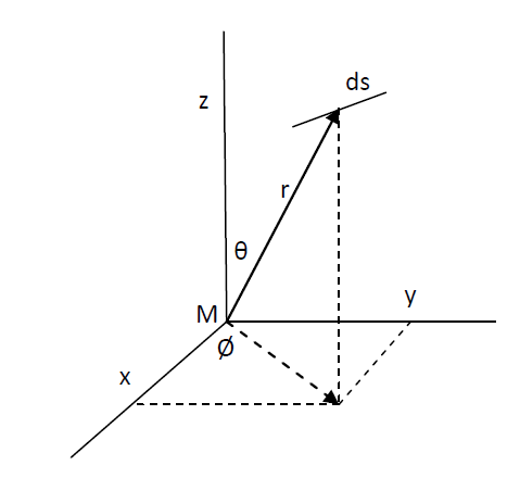
3.3.1 The chosen coordinate system and the local structure of space
We work here with a Euclidean coordinate system, which can be interpreted as a Cartesian system (\(t, x, y, z \)) or,as in the Schwarzschild solution,a polar system (\(t, r, θ, ∅ \)). In the polar case, the path that a particle follows depends on all four coordinates.
The Schwarzschild metric assigns to each differential a coefficient that is a function of \(r\) and \(θ\), but independent of \(t\) and \(∅\). This reflects the spherical symmetry around the mass \(M\): a rotation about the center does not change the physical situation.
It is important to realize that these coordinates are hypothetical: they are defined as if they exist in a flat, non-curved spacetime. Schwarzschild found an explicit formula that describes the curvature of spacetime around a point mass. This formula relates the infinitesimal line element \(ds\) (the distance in spacetime between two neighboring events) to the chosen coordinate system.
Although spacetime is curved, we can treat it locally,in an infinitesimally small region,as flat. Within such a small region, we may treat the coordinates \(c dt\), \(dr\), \(dθ\), and \(d∅\) as mutually orthogonal and linear. The coefficients in the metric can then be regarded as constant. If we move to another location, these properties remain locally valid, but with modified coefficients due to changes in \(r\) and \(θ\).
By integrating \(ds\) along a path, that is, summing all infinitesimal steps, we obtain the complete trajectory of the particle in curved spacetime.
3.3.2 The Schwarzschild Metric and the Role of Proper Time
As discussed earlier, the Schwarzschild metric in polar coordinates has the form:
Here, \( d s^2 \) describes the squared interval in spacetime between two neighboring events.
For greater compactness, we introduce the function:
so that the metric can be elegantly rewritten as:
Here \( d\tau \) is the proper time: the time measured by a clock moving along with the object. This is the actual duration experienced by an observer along their own worldline.
The coordinate time \( dt \), on the other hand, belongs to a hypothetical frame in which no mass is present, an ideal “flat” reference frame. Strictly speaking, \( dt \) is not directly measurable, except in the limit \( r \to \infty \), where \( \sigma \to 1 \) and spacetime becomes flat.
Locally, at a fixed value of \( r \), the Schwarzschild metric relates coordinate time and proper time via a simple relation:
where \( \sigma \) depends on the position \( r \).
3.3.3 Distance Traveled, Velocity, and the Relation to the Schwarzschild Metric
In Schwarzschild spacetime, the infinitesimal spatial distance Δdistance between two events is given by:
Where, as mentioned earlier:
The corresponding time interval is the proper time at location \( r \) :
This yields for the (local) velocity \( v \) of a particle in the frame:
This explicitly takes into account the curvature of spacetime.
If we substitute this expression back into the compact form of the Schwarzschild metric (equation (\ref{eq:R18})), we obtain:
which simplifies to:
or, written more compactly:
where:
This derivation shows how both spatial and temporal curvature together determine the dynamics of a moving particle.
3.3.4 Relation between Proper Time and Coordinate Time \(dt\)
From the previous derivation (equation (\ref{eq:R25})), the relation between proper time \( d\tau \) and coordinate time \( dt \) follows directly:
Where:
Here, \(\sigma\) is a measure of gravitational time dilation (due to the mass \(M\)) and \(\gamma\) is the Lorentz factor from special relativity.
Since \(\gamma \ge 1\) (because \(v \le c\)) and \(\sigma \le 1\) (since \( r \ge 2GM/c^2 \)), it follows that:
This means that the proper time of the moving object always elapses more slowly than the coordinate time in the reference frame.
Since both \(\sigma\) and \(\gamma\) are constant over the interval considered (they depend only on \( r \) and \( v \), not on \( t \)), we can integrate this relation straightforwardly:
where \(\tau\) is the elapsed proper time and \( t \) is the elapsed coordinate time.
Thus:
- \(t\) is the coordinate time of an external observer (for example, someone far away from the gravitational field).
- \(\tau\) is the proper time of the particle itself.
And:
- \(\frac{dt}{d\tau}\) = rate at which coordinate time flows relative to the particle’s proper time.
- \(\frac{dt}{d\tau}\) is not a velocity in meters per second like \(\frac{dr}{dt}\), but a relative “time rate” between the observer’s coordinate time and the particle’s proper time.
- It does, however, play the same role in the Lagrangian as a kinetic term: the square \(dt^2\) appears in the energy-like conserved quantity.
3.3.5 Behavior of a Photon in the Schwarzschild Metric
For a photon, the proper time \( d\tau \) is zero, since a photon always moves at the speed of light:
From this it follows that the spatial distance traveled by the photon is given by:
The effective speed of light \( v \) with respect to the chosen coordinate system can now be determined:
Here, \(\Delta \textit{time} = \sigma dt\), as discussed earlier.
3.3.6 Interpretation
- In the numerator we find the 'normal' spatial distance traveled by the photon.
- In the denominator we see that time is affected by a factor \(\sigma\): the clock at a given location runs more slowly due to the gravitational influence.
This shows that, when measured in coordinate time \( dt \), the speed of light is effectively lower than \( c \) in the presence of gravity. In the local (comoving) frame, the photon still moves at the constant speed \( c \).
3.3.7 Alternative Description of Photon Motion
We can also rewrite the relation between distance traveled and elapsed time as follows:
Here we note:
- The spatial distance is increased by a factor \(\sigma^{-2}\) (since \(\sigma \le 1\)).
- At the same time, the coordinate time \( dt \) remains unchanged.
3.3.8 Consequence
Because of this increased distance in the numerator, while the time in the denominator remains unchanged, the speed of light in the coordinate system appears smaller than the universal speed of light \( c \).
3.3.9 Summary Picture
From the perspective of the 'universal' coordinate system:
- A photon moves along a curved path in curved spacetime, and
- The effective speed of the photon between two coordinate points (for example from A to B) is less than \( c \).
In the relation:
it can be seen that the speed of light is effectively modified by the factor \(\sigma^2\).
3.3.10 Behavior
This means physically that:
- The intrinsic speed of the photon remains \( c \) along its worldline.
- But the projection of its motion onto the coordinate system appears as a lower speed due to the curvature of spacetime.
In other words:
Because the path length is greater than the 'straight-line distance', we have \( v < c \) when measured in coordinate time.
3.3.11 Relation between Local Time on Earth and Universal Frame Time
As noted earlier, coordinate time \( dt \) is a hypothetical time, defined in a massless environment or at infinite distance \( r = \infty \). Since our measurements are performed from Earth, we must establish a relation between(see also chapter 4.6):
- the proper time \( d\tau_{\textit{earth}} \) as measured by a clock on Earth, and
- the coordinate time \( dt \) from the universal reference frame.
As derived earlier (see also equation (\ref{eq:R34})), we have:
Or, equivalently:
where:
- \(\sigma_{\textit{earth}} =\sqrt{ 1 - \frac{2GM}{c^2 r_{\textit{earth}}}}\) is the gravitational time dilation factor,
- \(\gamma_{\textit{earth}} = \frac{1}{\sqrt{1 - v_{\textit{earth}}^2 / c^2}}\) is the special relativistic Lorentz factor (due to Earth's rotation).
3.3.12 Interpretation
Time on Earth is therefore slowed relative to the universal frame due to two effects:
- gravity (gravitational time dilation, via \(\sigma\)),
- motion of the Earth (special relativity, via \(\gamma\)).
For an observer moving with the Earth, proper time \( d\tau_{\textit{earth}} \) flows normally; each second remains a second. However, relative to the universal frame time \( dt \), local seconds run slightly slower.
3.3.13 Summary
- On Earth: proper time proceeds normally (i.e., according to \( d\tau \)).
- Relative to the universal frame: proper time is slowed due to gravitational and motion effects.
3.3.14 Behavior of a Photon in the Schwarzschild Metric
A special case arises when we consider a photon. Since a photon always travels at the speed of light \( c \) and has no rest mass, the proper time \( d\tau \) along its worldline is zero:
This also follows directly from the Schwarzschild metric:
From this we can derive that the spatial distance traveled \( \Delta \textit{distance} \) is:
and the speed of the photon is:
3.3.15 Remark
Although a photon would have a "zero distance" in its own (non-existent) rest frame, an external observer does observe a distance traveled along a curved path in spacetime.
3.3.16 Special Cases
- Radial motion of the photon (only r-direction, \( d\tau = d\theta = d\phi = 0 \))
Then the previous equation simplifies to:
\begin{align} c^2 = \sigma^{-4} \left(\frac{dr}{dt}\right)^2 \quad \end{align} - Circular motion in the equatorial plane \(\left( \theta = \pi/2 \right)\)
If the photon moves in a circular orbit around the mass \( M \) (\( d\tau = dr = d\theta = 0 \)), then:
\begin{align} v = c = \frac{r d\phi}{\sigma dt} \end{align}It follows that the angular velocity \( d\phi/dt \) depends on the distance \( r \) and the curvature factor \(\sigma\).
that is
3.3.17 At Large Distance
If \( r = \infty \), then
3.3.18 Summary
- For a photon, \( d\tau = 0 \) always holds.
- The relation between space and time is fully determined by the curvature factor \(\sigma\).
- In strongly curved spacetime (near mass), the behavior of a photon deviates significantly from what we intuitively expect in flat spacetime.
In general, at infinite distance the motion is straight and uniform, and thus the equation becomes:
3.3.19 Transformation to Cartesian Coordinates
The original approach by Schwarzschild was not in polar, but in Cartesian coordinates. The transformation results in:
where:
- \(\sigma =\sqrt{ 1 - \frac{2GM}{c^2 r}}\)
- \( r = \sqrt{x^2 + y^2 + z^2} \) is the usual radial distance.
3.3.20 Explanation
The first term \( \sigma^2 c^2 dt^2 \) describes the time component dependent on gravity. The second term \( dx^2 + dy^2 + dz^2 \) corresponds to flat spacetime. The third term corrects for the fact that time dilation also affects spatial components, depending on the direction in which we move relative to the mass \( M \).
3.3.21 Remark on Differentiating with Respect to t or τ
- Time \( t \) is the coordinate time, measured by an observer at infinite distance (or in a region without mass).
- Time \( \tau \) is the proper time, measured along the worldline of the moving object.
For the plane \( \theta = \pi/2 \) and dividing by \( c^2 d\tau^2 \):
or, rewriting using derivatives with respect to \(t\):
Then:
This shows how motion (velocities) and time dilation are related in curved spacetime.
3.3.22 Velocity with Respect to Local and Universal Time
The velocity with respect to the proper time \( \tau \) is:
and the Schwarzschild metric can be written in terms of \( v_{\textit{co}} \):
Or rewritten:
Approximation for small velocities \( (v_{co} \ll c) \) via a Taylor expansion:
With \( \gamma_{co} = \dfrac{1}{\sqrt{1 - \dfrac{v_{co}^2}{c^2}}} \).
3.3.23 Summary
- Schwarzschild originally worked in Cartesian coordinates.
- The Schwarzschild metric can be expressed in both spherical and Cartesian form.
- When interpreting motion, it is essential to distinguish between coordinate time \( t \) and proper time \( \tau \).
- For small velocities, the influence of spacetime curvature on time is small but measurable.
In general, a trajectory lies in a single plane. The polar system can then be chosen such that the equatorial plane coincides with the plane of motion (\( \theta = \pi/2 \)). If the trajectory is circular (\( r \) constant), then \( dr = 0 \) and we obtain:
We now present some additional considerations:
3.3.24 Addition 1: Interpretation of ds as a Line Element in Spacetime
It may be useful to view ds as an infinitesimally small line element in spacetime, whose length in meters can be measured by multiplying the travel time of a photon along that segment by the speed of light c. The line element ds is located at the origin of its own comoving reference frame. Within that frame, time is the only physical quantity that can be directly measured. Distance is measured via the travel time of the photon.
Thus:
where \( d\tau \) is the proper time recorded on a comoving clock.
We now introduce a second reference frame, for example the Schwarzschild frame, in which a central mass M is present. In this frame, we can determine the distance between the line element and the origin using external measuring instruments (such as lasers, rods, etc.).
Important:
To clarify the relation between proper time and Schwarzschild coordinates, we introduce two auxiliary quantities:
- \( c\Delta T \) — the time component of the interval in the external Schwarzschild frame, expressed as a length (in meters),
- \( \Delta X \) — the spatial component of that same interval.
This notation aligns with the usual expression of the Minkowski interval \( ds^2 = (c\Delta T)^2 - (\Delta X)^2 \), and makes the comparison with flat spacetime immediately clear.
The time determination in this external frame is indirect: it depends on the relation given by the Schwarzschild metric and cannot be measured directly with a local clock.According to the Schwarzschild metric:
\( c^{2}d\tau^{2} = \left(c\Delta T\right)^{2} - \left( \Delta X \right)^{2} \)
\( \left(c\Delta T\right)^{2} = \left(1 - \dfrac{2GM}{c^{2}r}\right)c^{2}dt^{2} =c^{2}d\tau^{2} - \left( \Delta X \right)^{2} \)
where \( \Delta X \) is the spatial component:
\( \left( \Delta X \right)^{2} = \dfrac{1}{1 - \dfrac{2GM}{c^{2}r}}\,dr^{2} + r^{2}d\theta^{2} + r^{2}\sin^{2}\theta\,d\phi^{2} \)
It follows that:
\( c^{2}dt^{2} = \dfrac{\left(c\Delta T\right)^{2}}{1 - \dfrac{2GM}{c^{2}r}} \)
The relation between the theoretical time dt and the proper time \( d\tau \) can only be determined via this formula.
3.3.25 Addition 2: Worldline of a Particle in a Comoving Reference Frame
If we consider a particle in a comoving (local) reference frame, then the particle is at rest relative to that frame. The only path the particle follows in spacetime is along its own τ-axis: proper time.
However, we can describe the motion of the particle relative to an external (possibly moving) reference frame. In that case, we express the position of the particle in coordinates \((t, x, y, z)\) of that other frame.
The worldline of the particle, the path it follows through spacetime, is then entirely a function of \(\tau\):
The four coordinates are thus functions of the proper time \(\tau\).
3.3.26 Example: Time Difference Between the Poles and the Equator
We calculate the time difference at the Earth's surface between time at the poles and at the equator, caused by relativistic effects.
Starting from the Schwarzschild metric:
3.3.27 At the Poles
At the poles:
- \(dr = 0\) (no radial motion),
- \(θ = 0\),
- \(dθ = 0\),
- \(sin θ = 0\).
3.3.28 At the Equator
At the equator:
- \(dr = 0\),
- \(θ = \pi/2\),
- \(dθ = 0\),
- \(sinθ = 1\)
We rewrite this:
Thus:
3.3.29 Practical Calculation
The rotational velocity at the equator is approximately:
3.3.30 Interpretation
A clock at the equator ticks slightly slower than a clock at the poles. Over a period of 100 years the difference would amount to approximately:
100 years * 1.2·10⁻¹² ≈ 3.75 milliseconds
3.3.31 Conclusion
A person who has lived 100 years at the North Pole would (theoretically) be 3.75 milliseconds older than someone who stayed at the equator, assuming all other conditions remain equal.
3.3.32 Addition 3: The Schwarzschild Coefficient and Escape Velocity
Let us pay special attention to the factor:
This expression resembles the well-known formula for escape velocity, which determines the minimum speed a mass must have to escape another mass (for example, the Earth).
3.3.33 Calculation of the Minimum Escape Velocity
Consider a mass m launched from an object with mass M (for example, the Earth):
- The kinetic energy of m: \begin{align} E_{\text{kin}} = \frac{1}{2} m v^2\end{align}
- The gravitational force acting on m: \begin{align} F = \frac{G M m}{r^2}\end{align}
- The work required to move the mass m from r to infinity
(where gravitational influence is zero) is:
\begin{align} W = \int_r^\infty F \, ds =\int_r^\infty \frac{G M m}{s^2} \, ds = GMm \left[ -\frac{1}{s} \right]^{\infty}_{r} \end{align}\begin{align} = GMm \left[ \frac{1}{s} \right]_{\infty}^{r} = G M m \left[\frac{1}{r}-\frac{1}{\infty}\right]=G\frac{M m}{r} \end{align}
where r is the distance to the center of mass M.
3.3.34 The Maximum Speed: Light
The maximum speed an object can reach is the speed of light c. If v = c, then the corresponding distance becomes:
3.3.35 Relation to the Schwarzschild Metric
In the Schwarzschild metric, this radius appears in the factor:
- At large distances \(r \to \infty\), the factor approaches 1.
- Near the Schwarzschild radius \(r = R_s\), the factor becomes 0.
3.3.36 Remark
If \(r\) becomes smaller than \(R_s\), the factor would become negative. The physical meaning of this requires deeper analysis within relativistic black hole theory and lies beyond the scope of this discussion.
3.3.37 Key Points and Intuition
- In general relativity, geometry replaces force: mass curves spacetime instead of generating a force field.
- The Schwarzschild metric describes this curvature around a spherically symmetric mass and applies outside the mass, where \(T_{\mu \nu}=0\).
- A test particle moving in this field feels no force, but follows a geodesic, the “straightest” path in curved spacetime.
- The metric in spherical coordinates:
\begin{align} ds^2 = c^2 d\tau^2 = \sigma^2 c^2 dt^2 − \sigma^{-2} dr^2 − r^2 d\theta^2 − r^2 sin^2 \theta \, d\phi^2 \end{align}with\begin{align} \sigma^2 = 1 - \frac{2GM}{c^2 r}\end{align}
- Coordinate time \(dt\) applies in the asymptotically flat (hypothetical) frame at \(r \to \infty\); proper time \(d\tau\) is measured by a clock comoving with the object.
Intuitively: Einstein states that mass affects the measurement structure of space and time itself. A freely falling object does not move “due to a force,” but follows the path dictated by the geometry of spacetime, similar to a pebble rolling on a curved surface.
- Time runs slower closer to a mass (via \(σ < 1)\).
- Space is stretched in the radial direction.
- For a moving object, the metric relates \(dτ\) to \(dt\) and its velocity \(v\):
\begin{align} dτ =\frac{ σ}{γ} dt \text{, with } γ =\frac{ 1 }{\sqrt{\left(1 - v²/c²\right)}}\end{align}
Table: Quantities and Physical Meaning in the Schwarzschild Metric
| Quantity | Physical interpretation |
|---|---|
\begin{align} \sigma=\sqrt{\left(1 - \frac{2GM}{c²r}\right)}\end{align}
| Gravitational time dilation factor |
\begin{align} dτ\end{align}
| Proper time: measured by a local clock |
\begin{align} dt\end{align}
| Coordinate time: measured in an asymptotically flat reference frame |
\begin{align} v\end{align}
| Local velocity, derived from spatial coordinates and dt |
\begin{align} ds^2 = c^2 dτ^2\end{align}
| Four-dimensional interval (invariant): spacetime element |
\begin{align} R_s = \frac{2GM}{c^2}\end{align}
| Schwarzschild radius: where σ = 0, event horizon |
3.3.38 Special Cases and Effects
- Photons:
- Follow a trajectory with \(dτ = 0\): they experience no proper time.
- The effective speed of light in coordinate time is less than \(c\) (but locally \(v = c\)).
- Object at rest near a mass:
- Time dilation via \(dτ = \frac{σ}{γ} dt\): the smaller \(r\), the slower the clock.
- Moving object (e.g. circular orbit):
- Both gravitational and kinematic time dilation play a role.
- Velocity in Schwarzschild coordinates:
3.3.39 Application: Time on Earth vs. Time at Infinite Distance
- Time on Earth runs slower compared to universal coordinate time due to:
- gravity (via \( σ \)),
- Earth’s rotation (via \( γ \)).
- Result: over 100 years, a clock at the poles is ≈ 3.75 ms ahead of a clock at the equator (approximately).
3.3.40 Black Holes and Escape Velocity
- From Newtonian mechanics:
\begin{align} v_{\text{escape}} = \sqrt{\frac{2 G M}{r}} \Rightarrow R_s = \frac{2 G M}{c^2} \end{align}
- At \( r = R_{s} \), \( σ \to 0 \) (event horizon): nothing can escape.
- The Schwarzschild metric explicitly contains this boundary.
3.3.41 Final Insight
The Schwarzschild metric directly provides measurable predictions:
- Time dilation (e.g. GPS corrections)
- Light deflection (as measured during solar eclipses)
- Perihelion precession of Mercury
- Conditions for black hole formation
The Schwarzschild metric is therefore not an abstract mathematical object, but a physical machine that tells us how clocks run, how light bends, and how masses move, purely based on the geometry of space and time.
3.4 Experiments: Confirmation of General Relativity
General relativity is not only an elegant mathematical theory, but is also strongly supported by experiments and observations. Many of these experiments use the Schwarzschild solution as the basis for their theoretical predictions. The following experiments are discussed in this work:
- Hafele-Keating experiment (1971) (see chapter 4.1)
- Description: Atomic clocks were flown around the Earth in airplanes, both eastward and westward, and compared with clocks on the ground.
- Result: The measured time differences matched exactly the predictions of general relativity (both gravitational time dilation and velocity time dilation).
- Relation to Schwarzschild metric: Gravitational time dilation is directly derived from the Schwarzschild solution.
- Motion of particles in a gravitational field (see chapter 4.2)
- Description: The trajectories of satellites, planets, and other objects are precisely tracked.
- Result: The observed trajectories agree with predictions from Schwarzschild geometry, including small deviations from classical (Newtonian) predictions.
- Deflection of light near masses (see chapter 4.3)
- Description: During solar eclipses, measurements were made of how starlight is bent by the Sun’s gravity.
- Result: The measured deflection (by Eddington in 1919 and many later experiments) exactly matches the value predicted by the Schwarzschild metric.
- Physical significance: Demonstrates that light itself is affected by spacetime curvature.
- Precession of perihelia (Mercury) (see chapter 4.4)
- Description: Mercury’s orbit slowly rotates around the Sun; this precession cannot be fully explained by Newtonian gravity.
- Result: The remaining precession is exactly explained by the Schwarzschild solution.
- Historical significance: One of the first major successes of general relativity.
- Shapiro time delay (see chapter 4.5)
- Description: Radio waves traveling near the Sun take longer than expected in flat spacetime.
- Result: The additional time delay matches the prediction of the Schwarzschild metric.
- Application: Used in radar and communication satellites.
- Trajectory of a projectile in a strong gravitational field (see chapter 4.8)
- Description: Simulations and measurements of objects moving at high speed near massive bodies.
- Result: The trajectories deviate from Newtonian predictions but agree with Schwarzschild predictions.
Conclusion
In all these experiments, the results are in excellent agreement with the predictions of general relativity, as derived from the Schwarzschild metric. This provides strong confirmation of the correctness of Einstein’s theory.
Key Point
General relativity is not only a mathematically elegant theory, but is also experimentally confirmed with high precision. The Schwarzschild metric is key to understanding most classical tests of gravity.