Part II – Derivation of the General Theory of Relativity Derivation of the General Theory of Relativity
2 General Relativity General Relativity
Before Einstein formulated his celebrated special theory of relativity in 1905, he first considered only coordinate systems moving uniformly with respect to one another. The influence of masses — and therefore gravity — was not yet included.
Special relativity is built upon two fundamental postulates:
- The speed of light in vacuum is the same in every inertial frame and equals \( c = 299\,792\,458 \,\text{m/s} \).
- The laws of nature hold in every inertial (non‑accelerating) reference frame.
In Newtonian physics, time was assumed to be universal. Special relativity demonstrated that time intervals depend on the observer’s motion — an effect known as time dilation.
The length of an object also changes under motion: it decreases relative to its rest length, known as length contraction. Both phenomena are discussed in Appendix 7.
Einstein unified space and time into a single entity: spacetime spacetime
One of the most famous consequences of this theory is the mass–energy relation:
\[ E = mc^2 \]
Extending his theory to accelerating frames led Einstein in 1915 to the general theory of relativity general theory of relativity , where gravity is no longer treated as a force but as a manifestation of spacetime curvature.
2.1 The Equivalence Principle The Equivalence Principle
Newton formulated the law of gravitation: masses experience acceleration due to an attractive force. Gravity differs from electric and magnetic forces, but shares some similarities. We begin by examining how forces arise and what accelerations they produce.
2.1.1 Electric force Electric force
The electric force arises from charges \(q_1\) and \(q_2\), with magnitude given by Coulomb’s law:
\[ F = k_e \frac{q_1 q_2}{r^2} \]
2.1.2 Magnetic force Magnetic force
Magnetic forces also produce acceleration depending on the charge, magnetic field, and particle mass.
2.1.3 Gravitational force Gravitational force
The gravitational force between masses \(m_1\) and \(m_2\) is given by Newton’s law:
\[ F = G \frac{m_1 m_2}{r^2} \]
The equivalence of gravitational and inertial mass leads to uniform acceleration of all objects in a gravitational field:
\[ a = G \frac{M}{r^2} \]
2.1.4 Einstein’s thought experiment Einstein’s thought experiment
Two locally indistinguishable situations demonstrate the equivalence principle: standing on Earth vs inside an accelerating rocket. Gravity is then seen as curvature of spacetime, not a force.
2.1.6 Confirmation by Observation Confirmation by Observation
Arthur Eddington’s 1919 eclipse observations confirmed gravitational deflection of light, validating general relativity.
2.2 Curvature of Spacetime Curvature of Spacetime
Particles move along straight lines in empty space. Near a massive body, mass deforms spacetime. The particle follows a geodesic in this curved geometry.
2.2.1 From Force to Geometry From Force to Geometry
Einstein needed a coordinate-independent formulation describing how mass and energy influence geometry, leading to the Einstein field equations.
2.2.3 Vector Approach to Distance Vector Approach to Distance
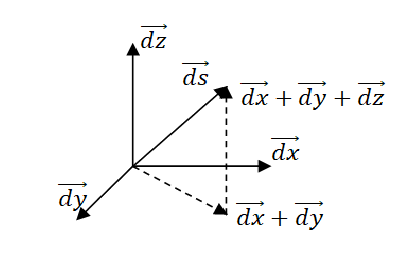
Differential displacement \(d\vec{s}\) is expressed as vector components along chosen axes. Magnitude:
\[ ds^2 = d\vec{s} \cdot d\vec{s} \]
Figure 2.3 illustrates decomposition of \(d\vec{s}\) along basis vectors Figure 2.3 Figure 2.3 – Decomposition of d⃗s along basis vectors .
2.2.4 Extension to Spacetime Extension to Spacetime
In four dimensions (one time + three spatial axes), the metric tensor \(g_{\mu\nu}\) encodes spacetime geometry: metric tensor Metric tensor
Spacetime interval:
\[ ds^2 = g_{\mu\nu} dx^\mu dx^\nu \]
The metric is symmetric (\( g_{\mu\nu} = g_{\nu\mu} \)), so only 10 independent components exist.
2.2.5 Key Insights Key Insights
- Particles move in straight lines in flat space (inertial motion).
- Mass curves spacetime; straight paths appear curved externally.
- Gravity = curvature; no force in Newtonian sense.
- Geodesics represent shortest or straightest paths in curved spacetime.
- Einstein’s challenge: coordinate-independent formulation → Einstein field equations.
2.2.6 Intuitive Explanation Intuitive Explanation
- Billiard ball on flat table → straight line.
- Heavy sphere on rubber sheet → smaller ball deviates from straight path.
- Falling objects follow shortest path in curved spacetime.
2.3 Covariant and Contravariant Vectors and Dual Vectors Covariant and Contravariant Vectors and Dual Vectors
In general relativity, the concepts of contravariant and covariant quantities appear frequently. In this section we explain these ideas and show how they arise from the way vectors and fields transform under a change of coordinate system.
As discussed earlier, physical quantities — such as vectors, tensors, and fields — must be independent of the chosen coordinate system. When we switch to a new system (for example by rotation or translation), the physical object remains the same, but its components change in a specific way. They transform according to well‑defined rules, depending on whether the object is covariant or contravariant.
2.3.1 Scalar Quantities, Vectors, and Fields Scalar Quantities, Vectors, and Fields
A scalar quantity, such as temperature, has a value at each point but no direction. A collection of scalar values over space forms a scalar field.
When such a field varies in a direction‑dependent way (for example, a temperature gradient), we can take its derivative. This derivative behaves like a vector, and in this specific context we call it a dual vector.
A dual vector depends on the chosen coordinate system: under a transformation, its components change in such a way that the physical meaning remains consistent. Because these components transform “with” the coordinate system, they are called covariant.
A “regular” vector (such as velocity or acceleration) behaves differently: when the coordinate system changes, the underlying vector remains physically the same, but its components change in the opposite manner relative to the basis vectors. Such vectors are called contravariant.
2.3.1.1 Notation and Definitions Notation and Definitions
To distinguish between the two types of vectors, the following notation is used:
- A contravariant vector carries an upper index: \( A^{\mu} \).
- A covariant vector carries a lower index: \( A_{\mu} \).
They are related through the metric tensor \( g_{\mu\nu} \) via:
\[ A_{\mu} = g_{\mu\nu} A^{\nu} \]
Contracting a contravariant vector with its covariant counterpart yields a scalar invariant:
\[ A^{\mu} A_{\mu} = I \]
This expression means that the inner product of a vector with its dual (or “lowered”) version results in a quantity \( I \) that remains invariant under coordinate transformations. This number \( I \) can be interpreted as the norm or the squared interval in spacetime, depending on its sign:
- Timelike: \( I < 0 \)
- Spacelike: \( I > 0 \)
- Lightlike: \( I = 0 \)
This classification highlights the central role of the metric tensor: it determines not only how vector components transform, but also how distances, lengths, and causal structures are defined in curved spacetime.
2.3.2 Transformations Between Coordinate Systems Transformations Between Coordinate Systems
Suppose we work in a coordinate system with coordinates \( x^{m} \) (where \( m = 0,1,2,3 \)), and we move to a new coordinate system with coordinates \( y^{n} \). The relation between the two systems is given by:
\[ y^{n} = \frac{\partial y^{n}}{\partial x^{0}} x^{0} + \frac{\partial y^{n}}{\partial x^{1}} x^{1} + \frac{\partial y^{n}}{\partial x^{2}} x^{2} + \frac{\partial y^{n}}{\partial x^{3}} x^{3} \]
In Einstein notation, where repeated indices (from 0 to 3) are summed automatically, this becomes:
\[ y^{n} = \frac{\partial y^{n}}{\partial x^{m}} x^{m} \]
2.3.2.1 Example: Derivative of a Scalar Function Example: Derivative of a Scalar Function
Consider a scalar function \( \varphi \). Its differential is:
\[ d\varphi = \frac{\partial \varphi}{\partial x^{m}} dx^{m} \]
Fully expanded:
\[ d\varphi = \frac{\partial \varphi}{\partial x^{0}} dx^{0} + \frac{\partial \varphi}{\partial x^{1}} dx^{1} + \frac{\partial \varphi}{\partial x^{2}} dx^{2} + \frac{\partial \varphi}{\partial x^{3}} dx^{3} \]
In the new coordinate system \( y^{n} \), we use the chain rule to transform the derivative components:
\[ \frac{d\varphi}{dy^{n}} = \frac{\partial \varphi}{\partial x^{m}} \frac{dx^{m}}{dy^{n}} \]
From this we see that the components transform as:
\[ A_{n}(y) = \frac{dx^{m}}{dy^{n}} B_{m}(x) \tag{1} \]
where:
- \( A_{n}(y) = \dfrac{d\varphi}{dy^{n}} \): the covariant vector in the \( y \)-system,
- \( B_{m}(x) = \dfrac{\partial \varphi}{\partial x^{m}} \): the covariant vector in the \( x \)-system.
This is a covariant transformation.
2.3.2.1.1 Fully Expanded (Matrix Form) Fully Expanded (Matrix Form)
In matrix form, expression (1) becomes:
\[ \begin{pmatrix} A_{0} \\ A_{1} \\ A_{2} \\ A_{3} \end{pmatrix}_{y} = \begin{pmatrix} \dfrac{dx^{0}}{dy^{0}} & \dfrac{dx^{1}}{dy^{0}} & \dfrac{dx^{2}}{dy^{0}} & \dfrac{dx^{3}}{dy^{0}} \\ \dfrac{dx^{0}}{dy^{1}} & \dfrac{dx^{1}}{dy^{1}} & \dfrac{dx^{2}}{dy^{1}} & \dfrac{dx^{3}}{dy^{1}} \\ \dfrac{dx^{0}}{dy^{2}} & \dfrac{dx^{1}}{dy^{2}} & \dfrac{dx^{2}}{dy^{2}} & \dfrac{dx^{3}}{dy^{2}} \\ \dfrac{dx^{0}}{dy^{3}} & \dfrac{dx^{1}}{dy^{3}} & \dfrac{dx^{2}}{dy^{3}} & \dfrac{dx^{3}}{dy^{3}} \end{pmatrix} \begin{pmatrix} B_{0} \\ B_{1} \\ B_{2} \\ B_{3} \end{pmatrix}_{x} \]
2.3.2.2 Contravariant Transformation Contravariant Transformation
For contravariant vectors, the transformation rule is the opposite of the covariant case:
\[ W^{n}(y) = \frac{dy^{n}}{dx^{m}} B^{m}(x) \]
Fully expanded in matrix form:
\[ \begin{pmatrix} W^{0} \\ W^{1} \\ W^{2} \\ W^{3} \end{pmatrix}_{y} = \begin{pmatrix} \dfrac{dy^{0}}{dx^{0}} & \dfrac{dy^{0}}{dx^{1}} & \dfrac{dy^{0}}{dx^{2}} & \dfrac{dy^{0}}{dx^{3}} \\ \dfrac{dy^{1}}{dx^{0}} & \dfrac{dy^{1}}{dx^{1}} & \dfrac{dy^{1}}{dx^{2}} & \dfrac{dy^{1}}{dx^{3}} \\ \dfrac{dy^{2}}{dx^{0}} & \dfrac{dy^{2}}{dx^{1}} & \dfrac{dy^{2}}{dx^{2}} & \dfrac{dy^{2}}{dx^{3}} \\ \dfrac{dy^{3}}{dx^{0}} & \dfrac{dy^{3}}{dx^{1}} & \dfrac{dy^{3}}{dx^{2}} & \dfrac{dy^{3}}{dx^{3}} \end{pmatrix} \begin{pmatrix} B^{0} \\ B^{1} \\ B^{2} \\ B^{3} \end{pmatrix}_{x} \]
2.3.3 Transformation Behaviour of Basis Vectors Transformation Behaviour of Basis Vectors
In tensor calculus, it is important not only to understand how the components of a vector transform under a coordinate transformation, but also how the associated basis vectors themselves transform.
- \( \vec e_{m} = \dfrac{\partial}{\partial x^{m}} \)
- \( \vec f_{n} = \dfrac{\partial}{\partial y^{n}} \)
The relation between basis vectors in different coordinate systems follows from the chain rule:
\[ \frac{\partial}{\partial x^{m}} = \frac{\partial y^{n}}{\partial x^{m}} \frac{\partial}{\partial y^{n}} \;\Rightarrow\; \vec e_{m} = \frac{\partial y^{n}}{\partial x^{m}} \vec f_{n} \]
This shows that basis vectors transform covariantly: they change along with the coordinate system. The components of contravariant vectors must therefore transform in the opposite way to keep the physical vector invariant.
2.3.3.1 Note on Einstein Notation Note on Einstein Notation
Einstein notation uses repeated indices (so‑called dummy indices), which are automatically summed over the values 0 through 3:
\[ A^{\mu} B_{\mu} = \sum_{\mu=0}^{3} A^{\mu} B_{\mu} \]
In this section, many expressions have been written out explicitly to clarify the meaning of this notation. In later chapters, we will use the compact Einstein notation more frequently.
2.3.4 Key Points
-
Scalars versus vectors:
Scalars versus vectors
- A scalar quantity (such as temperature) does not change under a coordinate transformation.
- A vector has both magnitude and direction. Its components do change under transformation, depending on the type of vector.
- Contravariant
vectors
Contravariant vectors
(such as position or velocity vectors \( W^{n} \)):
- Transform opposite to the basis vectors to keep the physical vector unchanged.
- Transformation rule: \[ W^{n}(y) = \frac{dy^{n}}{dx^{m}} B^{m}(x) \]
- Covariant vectors
Covariant vectors
(such as dual vectors \( A_{n} \)):
- Transform along with the coordinate system.
- Transformation rule: \[ A_{n}(y) = \frac{dx^{m}}{dy^{n}} B_{m}(x) \]
- Duality:
Duality
- Covariant vectors are linear functions acting on vectors; they belong to the dual vector space.
- Raising and lowering indices:
Raising and lowering indices
- Using the metric tensor \( g_{\mu\nu} \), we can convert between covariant and contravariant vectors: \[ A_{\mu} = g_{\mu\nu} A^{\nu}, \quad A^{\mu} = g^{\mu\nu} A_{\nu} \]
2.3.5 Intuitive Explanation
Intuitive ExplanationImagine standing on a hillside and measuring the slope in different directions. The hill itself does not change when you rotate your axes, but the numerical values you assign to the slope do. This is precisely the essence of tensor transformations: the physical direction of a vector remains the same, but the coordinates used to describe it depend on the chosen system.
The metric acts as a kind of converter between the two types of vectors. You can think of the metric as a ruler that measures differently in each direction, depending on the local curvature of spacetime.
Comparison Table Comparison Table
| Property | Contravariant | Covariant |
|---|---|---|
| Index position | Upper \( A^{\mu} \) | Lower \( A_{\mu} \) |
| Transforms… | Opposite to basis | Along with basis |
| Example | Position, velocity | Gradient, differential |
| Origin | Direction in space | Directional derivative of a scalar field |
2.4 Covariant and Contravariant Transformations of Tensors Covariant and Contravariant Transformations of Tensors
In general relativity — and tensor analysis more broadly — covariant, contravariant, and mixed tensors play a central role. The way these tensors transform under a change of coordinates is essential for expressing physical laws in a coordinate‑independent manner. In this section we discuss the transformation properties of the different types of tensors.
The transformation rules presented here are direct extensions of the vector transformation rules from the previous section.
2.4.1 Covariant Tensors Covariant Tensors
A covariant tensor has one or more lower indices, such as \( T_{mn} \), and can be constructed from the product of covariant vectors \( A_{m} \) and \( B_{n} \).
The transformation of a covariant tensor from a coordinate system \( x \) to a new system \( y \) is:
\[ T_{mn}(y) = A_{m}(y) B_{n}(y) = \frac{dx^{r}}{dy^{m}} A_{r}(x)\, \frac{dx^{s}}{dy^{n}} B_{s}(x) = \frac{dx^{r}}{dy^{m}} \frac{dx^{s}}{dy^{n}} T_{rs}(x) \]
2.4.2 Contravariant Tensors Contravariant Tensors
A contravariant tensor has one or more upper indices, such as \( T^{mn} \), and can be constructed from contravariant vectors \( A^{m} \) and \( B^{n} \).
The transformation is opposite to that of the covariant tensor:
\[ T^{mn}(y) = A^{m}(y) B^{n}(y) = \frac{dy^{m}}{dx^{r}} A^{r}(x) \frac{dy^{n}}{dx^{s}} B^{s}(x) = \frac{dy^{m}}{dx^{r}} \frac{dy^{n}}{dx^{s}} T^{rs}(x) \]
2.4.3 Mixed Tensors Mixed Tensors
A mixed tensor contains both upper and lower indices, for example \( T^{m}{}_{n} \). Such a tensor may arise from the product of a contravariant vector \( A^{m} \) and a covariant vector \( B_{n} \).
The corresponding transformation rule is:
\[ T^{m}{}_{n}(y) = \frac{dy^{m}}{dx^{r}} \frac{dx^{s}}{dy^{n}} T^{r}{}_{s}(x) \]
2.4.4 Key Points and Intuition Key Points and Intuition
- A tensor is characterized by its rank (number of indices) and the type of indices it carries (upper or lower).
- Tensors are the natural language for formulating physical laws that remain independent of the chosen coordinate system.
- The transformation properties of a tensor ensure that its physical meaning is preserved under coordinate changes.
Rank and Notation Rank and Notation
- A rank‑0 tensor is a scalar quantity, such as temperature or mass. It does not change under coordinate transformations.
- A vector is a rank‑1 tensor and can appear in two forms:
- Contravariant: written with an upper index, e.g. \( V^{m} \).
- Covariant: written with a lower index, e.g. \( V_{m} \).
- A rank‑2 tensor has several possible forms:
- Fully covariant: \( T_{\mu\nu} \),
- Fully contravariant: \( T^{\mu\nu} \),
- Mixed: \( T^{\mu}{}_{\nu} \), and so on.
Transformation Properties Transformation Properties
A tensor is defined by the way its components transform under a change of coordinates. These transformation rules ensure that tensors retain their physical meaning regardless of the coordinate system:
- Covariant components (lower indices, e.g. \( T_{\mu\nu} \)) transform with derivatives from the old to the new coordinates.
- Contravariant components (upper indices, e.g. \( T^{\mu\nu} \)) transform with derivatives from the new to the old coordinates.
- Mixed tensors combine both rules (e.g. \( T^{\nu}{}_{\mu} \)), depending on the position of the indices.
An important example is the metric tensor \( g_{\mu\nu} \), which allows us to raise or lower indices:
\[ T_{\mu} = g_{\mu\nu} T^{\nu} \]
Physical Relevance Physical Relevance
The fundamental equations of physics — such as the Einstein field equations in general relativity — are formulated in terms of tensors. This ensures invariance under coordinate transformations, a crucial feature of any covariant theory. It guarantees that physical laws retain their form regardless of the coordinate system and that the underlying geometry is described consistently.
Intuitive Picture Intuitive Picture
You can compare tensor transformations to redrawing a map:
- Imagine a topographic map with hills, valleys, and wind directions.
- You rotate the map by 30°, but the landscape does not change — only the coordinates used to describe it do.
Tensors behave like measurable structures in that world:
- A vector arrow on the map (e.g. wind direction) receives new coordinate components after rotation, even though its physical direction is unchanged.
- A gradient (e.g. slope of the terrain) still points uphill, but its components change depending on the new axes.
This is how tensors behave under transformations: their geometric or physical meaning remains the same, but their components change according to the chosen coordinate system.
Transformation Overview Transformation Overview
| Tensor Type | Index Notation | Transforms As… |
|---|---|---|
| Scalar | \( \phi \) | Remains unchanged |
| Contravariant vector | \( V^{\mu} \) | \( \dfrac{\partial y^{\mu}}{\partial x^{\nu}} V^{\nu} \) |
| Covariant vector | \( V_{\mu} \) | \( \dfrac{\partial x^{\nu}}{\partial y^{\mu}} V_{\nu} \) |
| Covariant tensor | \( T_{\mu\nu} \) | Twice the covariant rule |
| Contravariant tensor | \( T^{\mu\nu} \) | Twice the contravariant rule |
| Mixed tensor | \( T^{\mu}{}_{\nu} \) | Combination of both |
2.5 The Christoffel Symbol and the Covariant Derivative The Christoffel Symbol and the Covariant Derivative
To describe gravity as a geometric phenomenon, Einstein needed a mathematical framework to express the curvature of spacetime. Instead of forces, general relativity introduces structure into spacetime itself, with the Christoffel symbol playing a central role. This symbol describes how basis vectors change and forms the foundation of the covariant derivative, which is required for consistent differentiation in curved space.
2.5.1 Basic Definition of the Christoffel Symbol Basic Definition of the Christoffel Symbol
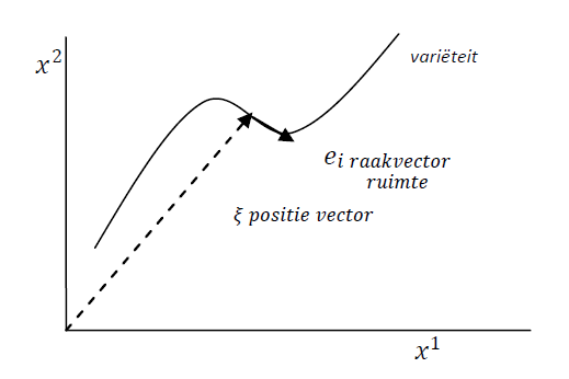
Consider a coordinate system \( x^{i} \) with an associated position vector \( \boldsymbol{\xi}(x^{i}) \), pronounced “ksi”, representing a spatial manifold. We define the basis vectors in the tangent space as the partial derivatives of \( \boldsymbol{\xi} \):
\[ e_{i} = \frac{\partial \boldsymbol{\xi}}{\partial x^{i}} \]
The derivative of this basis vector with respect to another coordinate \( x^{j} \) indicates how the direction of the basis vector changes in space:
\[ \frac{\partial e_{i}}{\partial x^{j}} = \frac{\partial^{2} \boldsymbol{\xi}}{\partial x^{i} \partial x^{j}} \]
This second derivative can be expressed as a linear combination of the basis vectors themselves:
\[ \frac{\partial e_{i}}{\partial x^{j}} = \Gamma^{k}{}_{ij}\, e_{k} \tag{2.5.1} \]
Here \( \Gamma^{k}{}_{ij} \) is the Christoffel symbol of the second kind. It describes how the basis vectors change, and therefore encodes the curvature of space. If this derivative is zero, the basis vectors do not change direction and the space is flat.
2.5.1.1 Vector Interpretation of Directional Change Vector Interpretation of Directional Change
The basis vectors \( e_{i} \) belong to the tangent space at a point of the manifold. The derivative in equation (2.5.1) tells us how this basis changes in the direction of \( x^{j} \). If \( \partial e_{i} / \partial x^{j} \neq 0 \), the space is curved.
Fully expanded, equation (2.5.1) becomes:
\[ \frac{\partial e_{i}}{\partial x^{j}} = \Gamma^{0}{}_{ij} e_{0} + \Gamma^{1}{}_{ij} e_{1} + \Gamma^{2}{}_{ij} e_{2} + \Gamma^{3}{}_{ij} e_{3}. \]
From this point onward, we omit the vector arrow on \( e_{i} \) for readability.
2.5.1.2 Derivation of the Christoffel Symbol Derivation of the Christoffel Symbol
Using the duality of basis vectors, we take the inner product with the dual basis vector \( e^{k} \):
\[ e^{k} \cdot e_{k} = 1 \tag{2.5.2} \]
Multiplying both sides of equation (2.5.1) by \( e^{k} \) yields:
\[ \Gamma^{k}{}_{ij} = e^{k} \cdot \frac{\partial e_{i}}{\partial x^{j}} \tag{2.5.3} \]
This provides a direct definition of the Christoffel symbol.
2.5.1.3 Symmetry of the Lower Indices Symmetry of the Lower Indices
In a smooth manifold, the order of differentiation does not matter (\( \partial_{i}\partial_{j} = \partial_{j}\partial_{i} \)), so:
\[ \frac{\partial e_{i}}{\partial x^{j}} = \frac{\partial e_{j}}{\partial x^{i}} \;\Rightarrow\; e^{k} \cdot \frac{\partial e_{i}}{\partial x^{j}} = e^{k} \cdot \frac{\partial e_{j}}{\partial x^{i}} \Rightarrow \Gamma^{k}{}_{ij} = \Gamma^{k}{}_{ji}. \tag{2.5.4} \]
Thus, the Christoffel symbol is symmetric in its lower indices: \( \Gamma^{k}{}_{ij} = \Gamma^{k}{}_{ji} \).
2.5.1.4 Derivation via the Coordinate Transformation
Derivation via the Coordinate TransformationConsider again
\[ e_{k} = \frac{\partial \boldsymbol{\xi}}{\partial x^{k}} \quad\Rightarrow\quad e^{k} = \frac{\partial x^{k}}{\partial \boldsymbol{\xi}}. \tag{2.5.5} \]
Substituting this into (2.5.3) gives
\[ \Gamma^{k}{}_{ij} = \frac{\partial x^{k}}{\partial \boldsymbol{\xi}} \cdot \frac{\partial^{2} \boldsymbol{\xi}}{\partial x^{i}\partial x^{j}}. \tag{2.5.6} \]
This expression shows that the Christoffel symbol is built from second derivatives of the coordinates, and is therefore directly related to the geometry of space-time.
2.5.1.5 Connection to the Metric Tensor
Connection to the Metric TensorThe metric tensor \( g_{ik} \) is defined as the inner product of the basis vectors:
\[ g_{ik} = e_{i} \cdot e_{k}. \tag{2.5.7} \]
Using the inverse metric \( g^{ik} \), we can convert basis vectors into one another:
\[ e^{i} = g^{ik} e_{k}, \qquad e_{i} = g_{ik} e^{k}. \tag{2.5.8} \]
2.5.1.6 Summary
Summary- The Christoffel symbol \(\Gamma^{i}{}_{jk}\) describes how basis vectors change in a curved space.
- It plays a central role in defining the covariant derivative, which will be discussed in the next section.
- The symmetry \(\Gamma^{i}{}_{jk} = \Gamma^{i}{}_{kj}\) follows from the commutativity of partial derivatives.
- The Christoffel symbol can be expressed both through coordinate derivatives and through the metric tensor, making it fundamentally linked to the structure of spacetime.
2.5.2 Covariant Derivative
Covariant DerivativeThe covariant derivative is a generalization of the ordinary derivative in flat space. In general relativity, this derivative must be modified so that it remains valid in curved spacetime. Einstein required his theory to be covariant: physical laws must retain the same form in every coordinate system.
To guarantee this, we define the covariant derivative \( \nabla \), which corrects the ordinary derivative with additional terms. This derivative satisfies
\[ \nabla_{s} g_{mn} = 0, \]
which defines the unique torsion-free, metric-compatible connection (the Levi–Civita connection).
2.5.2.1 Metric and Derivatives
Metric and DerivativesWe begin with the metric tensor (7): \[ g_{mn} = \mathbf{e}_m \cdot \mathbf{e}_n \tag{9} \]
Take the ordinary derivative with respect to \( x^s \): \[ \frac{\partial g_{mn}}{\partial x^s} = \frac{\partial (\mathbf{e}_m \cdot \mathbf{e}_n)}{\partial x^s} = \mathbf{e}_m \frac{\partial \mathbf{e}_n}{\partial x^s} + \mathbf{e}_n \frac{\partial \mathbf{e}_m}{\partial x^s} \tag{10} \]
Using the symmetry derived earlier (see equation 4), we may write: \[ \frac{\partial g_{mn}}{\partial x^s} = \mathbf{e}_m \frac{\partial \mathbf{e}_s}{\partial x^n} + \mathbf{e}_n \frac{\partial \mathbf{e}_s}{\partial x^m} \tag{11} \]
Bringing all terms to one side gives: \[ \frac{\partial g_{mn}}{\partial x^s} - \mathbf{e}_m \frac{\partial \mathbf{e}_s}{\partial x^n} - \mathbf{e}_n \frac{\partial \mathbf{e}_s}{\partial x^m} = 0 \tag{12} \]
2.5.2.2 Definition of the Covariant Derivative
Definition of the Covariant DerivativeThis relation motivates the definition of the covariant derivative of the metric: \[ \nabla_s g_{mn} = \frac{\partial g_{mn}}{\partial x^s} - \mathbf{e}_m \frac{\partial \mathbf{e}_s}{\partial x^n} - \mathbf{e}_n \frac{\partial \mathbf{e}_s}{\partial x^m} = 0 \tag{13} \]
We now express the tangent-space derivatives in terms of Christoffel symbols. From the previous section we know: \[ \Gamma^s{}_{nt} = \mathbf{e}^t \frac{\partial \mathbf{e}_s}{\partial x^n}, \qquad g_{mt} = \mathbf{e}_m \cdot \mathbf{e}_t \]
Substituting into (13) gives: \[ \nabla_s g_{mn} = \frac{\partial g_{mn}}{\partial x^s} - g_{mt} \Gamma^s{}_{nt} - g_{nt} \Gamma^s{}_{mt} = 0 \tag{15} \]
2.5.2.3 Cyclic Permutation
Cyclic PermutationApplying the same logic to permutations of the indices yields:
\[ \nabla_m g_{ns} = \frac{\partial g_{ns}}{\partial x^m} - g_{nt} \Gamma^m{}_{st} - g_{st} \Gamma^m{}_{nt} = 0 \tag{16} \]
\[ \nabla_n g_{sm} = \frac{\partial g_{sm}}{\partial x^n} - g_{st} \Gamma^n{}_{mt} - g_{mt} \Gamma^n{}_{st} = 0 \tag{17} \]
Now perform the operation: (17) + (16) − (15), using the symmetry \( \Gamma^i{}_{jk} = \Gamma^i{}_{kj} \) from equation (4). This yields:
\[ \frac{\partial g_{sm}}{\partial x^n} + \frac{\partial g_{ns}}{\partial x^m} - \frac{\partial g_{mn}}{\partial x^s} - 2 g_{st} \Gamma^n{}_{mt} = 0 \tag{18} \]
\[ g_{st} \Gamma^n{}_{mt} = \frac{1}{2} \left( \frac{\partial g_{sm}}{\partial x^n} + \frac{\partial g_{ns}}{\partial x^m} - \frac{\partial g_{mn}}{\partial x^s} \right) \tag{19} \]
2.5.2.4 Christoffel Symbol via the Metric
Christoffel Symbol via the MetricWe isolate \(\Gamma^n{}_{mt}\) by multiplying with the inverse metric \( g^{st} \):
\[ \Gamma^n{}_{mt} = \frac{1}{2} g^{st} \left( \frac{\partial g_{sm}}{\partial x^n} + \frac{\partial g_{ns}}{\partial x^m} - \frac{\partial g_{mn}}{\partial x^s} \right) \tag{20} \]
This expression gives the Christoffel symbols in terms of the metric tensor and its first derivatives.
2.5.2.5 Remarks
Remarks2.5.2.5.1 Covariance of the Metric
Covariance of the MetricWe confirm that the covariant derivative of the metric is indeed zero (see equation 8): \[ \nabla_\rho A_\mu = g_{\mu\nu} \nabla_\rho A^\nu \tag{20a} \]
Using \( A_\mu = g_{\mu\nu} A^\nu \) and the Leibniz rule:
\[ \nabla_\rho A_\mu = \nabla_\rho (g_{\mu\nu} A^\nu) = g_{\mu\nu} \nabla_\rho A^\nu + A^\nu \nabla_\rho g_{\mu\nu} \tag{20b} \]
Since (20a) and (20b) must give the same result:
\[ A^\nu \nabla_\rho g_{\mu\nu} = 0 \]
Because \( A^\nu \neq 0 \), it follows that: \[ \nabla_\rho g_{\mu\nu} = 0. \]
This confirms a fundamental property of the Levi–Civita connection.
2.5.2.5.2 Transformation Rule for Vector Components
Transformation Rule for Vector ComponentsThe standard transformation rule for a covariant tensor is: \[ T_{mn}^y = \frac{\partial x^r}{\partial y^m} \frac{\partial x^s}{\partial y^n} T_{rs}^x. \tag{35} \]
Substituting \(T_{rs}^x = \frac{\partial V_r^x}{\partial x^s}\): \[ T_{mn}^y = \frac{\partial x^r}{\partial y^m} \frac{\partial x^s}{\partial y^n} \frac{\partial V_r^x}{\partial x^s} = \frac{\partial x^r}{\partial y^m} \frac{\partial V_r^x}{\partial y^n}. \tag{36} \]
We now show that: \[ \frac{\partial V_m^y}{\partial y^n} \neq T_{mn}^y. \]
2.5.3.3 Computing \(\frac{\partial V_m^y}{\partial y^n}\)
ComputingUsing the transformation of vector components: \[ V_m^y = \frac{\partial x^r}{\partial y^m} V_r^x, \] we obtain: \[ \frac{\partial V_m^y}{\partial y^n} = \frac{\partial}{\partial y^n} \left( \frac{\partial x^r}{\partial y^m} V_r^x \right). \]
Applying the product rule: \[ \frac{\partial V_m^y}{\partial y^n} = \frac{\partial x^r}{\partial y^m} \frac{\partial V_r^x}{\partial y^n} + \frac{\partial^2 x^r}{\partial y^n \partial y^m} V_r^x. \tag{38} \]
Using the inverse transformation: \[ V_r^x = \frac{\partial y^a}{\partial x^r} V_a^y, \tag{39} \] we substitute into (38): \[ \frac{\partial V_m^y}{\partial y^n} = \frac{\partial x^r}{\partial y^m} \frac{\partial V_r^x}{\partial y^n} + \frac{\partial y^a}{\partial x^r} \frac{\partial^2 x^r}{\partial y^n \partial y^m} V_a^y. \tag{40} \]
2.5.3.4 Connection with Christoffel Symbols
Connection with Christoffel SymbolsRecall (from the earlier derivation of the Christoffel symbol): \[ \Gamma^n{}_{ma} = \frac{\partial y^a}{\partial x^r} \frac{\partial^2 x^r}{\partial y^n \partial y^m}. \]
Substituting into (40) gives: \[ \frac{\partial V_m^y}{\partial y^n} = \frac{\partial x^r}{\partial y^m} \frac{\partial V_r^x}{\partial y^n} + \Gamma^n{}_{ma} V_a^y. \]
Rearranging: \[ T_{mn}^y = \frac{\partial x^r}{\partial y^m} \frac{\partial V_r^x}{\partial y^n} = \frac{\partial V_m^y}{\partial y^n} - \Gamma^n{}_{ma} V_a^y. \tag{41} \]
Thus: \[ T_{mn}^y \neq \frac{\partial V_m^y}{\partial y^n}. \]
2.5.3.7.2 Final Formula
Final FormulaSince \(T_{\mu\nu} = A_\mu B_\nu\), we obtain: \[ \nabla_\alpha T_{\mu\nu} = \frac{\partial T_{\mu\nu}}{\partial x^\alpha} - T_{\beta\nu} \Gamma^\alpha{}_{\mu\beta} - T_{\mu\gamma} \Gamma^\alpha{}_{\nu\gamma} \tag{43} \]
2.5.3.7.3 Summary
SummaryThe covariant derivative of a covariant tensor \(T_{\mu\nu}\) consists of:
- the ordinary derivative \(\frac{\partial T_{\mu\nu}}{\partial x^\alpha}\),
- and two correction terms involving Christoffel symbols, one for each index of the tensor.
This ensures that \(\nabla_\alpha T_{\mu\nu}\) transforms as a tensor under coordinate transformations.
2.5.3.8 Covariant Differentiation of a Contravariant Tensor Covariant Differentiation of a Contravariant Tensor
We now extend the concept of covariant differentiation to a contravariant rank‑2 tensor. Such a tensor has two upper indices and transforms differently from a covariant tensor. We again apply the product rule and use the known formulas for covariant derivatives.
2.5.3.8.1 Starting Point Starting Point
Consider a contravariant tensor \(T^{\mu\nu}\) defined as the product of two contravariant vectors: \[ T^{\mu\nu} = A^\mu B^\nu \]
The covariant derivative of \(T^{\mu\nu}\) with respect to \(x^\alpha\) is: \[ \nabla_\alpha T^{\mu\nu} = B^\nu \nabla_\alpha A^\mu + A^\mu \nabla_\alpha B^\nu \tag{a} \]
Using the formulas for the covariant derivative of a contravariant vector (see 2.5.2.6.3): \[ \nabla_\alpha A^\mu = \frac{\partial A^\mu}{\partial x^\alpha} + \Gamma^\beta{}_{\alpha\mu} A^\beta \] \[ \nabla_\alpha B^\nu = \frac{\partial B^\nu}{\partial x^\alpha} + \Gamma^\gamma{}_{\alpha\nu} B^\gamma \]
Substituting into (a) gives: \[ \nabla_\alpha T^{\mu\nu} = B^\nu \frac{\partial A^\mu}{\partial x^\alpha} + A^\mu \frac{\partial B^\nu}{\partial x^\alpha} + A^\beta B^\nu \Gamma^\beta{}_{\alpha\mu} + A^\mu B^\gamma \Gamma^\gamma{}_{\alpha\nu} \]
Or equivalently: \[ \nabla_\alpha T^{\mu\nu} = \frac{\partial (A^\mu B^\nu)}{\partial x^\alpha} + T^{\beta\nu} \Gamma^\beta{}_{\alpha\mu} + T^{\mu\gamma} \Gamma^\gamma{}_{\alpha\nu} \]
2.5.3.8.2 Final Formula Final Formula
Since \(T^{\mu\nu} = A^\mu B^\nu\), we obtain: \[ \nabla_\alpha T^{\mu\nu} = \frac{\partial T^{\mu\nu}}{\partial x^\alpha} + T^{\beta\nu} \Gamma^\beta{}_{\alpha\mu} + T^{\mu\gamma} \Gamma^\gamma{}_{\alpha\nu} \tag{44} \]
2.5.3.8.3 Summary Summary
The covariant derivative of a contravariant tensor \(T^{\mu\nu}\) consists of:
- the ordinary derivative \(\frac{\partial T^{\mu\nu}}{\partial x^\alpha}\),
- and two correction terms involving Christoffel symbols, one for each upper index.
The order of indices in the Christoffel symbol is essential: the upper index indicates which tensor index is being corrected.
2.5.3.9 Covariant Differentiation of a Mixed Tensor Covariant Differentiation of a Mixed Tensor
We now examine how the covariant derivative applies to a mixed tensor — a tensor with one contravariant and one covariant index.
2.5.3.9.1 Starting Point Starting Point
Consider the mixed tensor \(T^\mu{}_\nu\), defined as: \[ T^\mu{}_\nu = A^\mu B_\nu \]
Its covariant derivative with respect to \(x^\alpha\) is: \[ \nabla_\alpha T^\mu{}_\nu = B_\nu \nabla_\alpha A^\mu + A^\mu \nabla_\alpha B_\nu \tag{a} \]
2.5.3.9.2 Using the Covariant Derivative Rules Using the Covariant Derivative Rules
Substitute the known expressions: \[ \nabla_\alpha A^\mu = \frac{\partial A^\mu}{\partial x^\alpha} + \Gamma^\beta{}_{\alpha\mu} A^\beta \] \[ \nabla_\alpha B_\nu = \frac{\partial B_\nu}{\partial x^\alpha} - \Gamma^\alpha{}_{\nu\gamma} B^\gamma \]
Substituting into (a) gives: \[ \nabla_\alpha T^\mu{}_\nu = \frac{\partial (A^\mu B_\nu)}{\partial x^\alpha} + T^\beta{}_\nu \Gamma^\beta{}_{\alpha\mu} - T^\mu{}_\gamma \Gamma^\alpha{}_{\nu\gamma} \]
2.5.3.9.3 Final Formula Final Formula
Since \(T^\mu{}_\nu = A^\mu B_\nu\), we obtain: \[ \nabla_\alpha T^\nu{}_\mu = \frac{\partial T^\nu{}_\mu}{\partial x^\alpha} + T^\beta{}_\mu \Gamma^\beta{}_{\alpha\nu} - T^\gamma{}_\nu \Gamma^\alpha{}_{\mu\gamma} \tag{45} \]
2.5.4 Key Points and Intuition
Key Points and Intuition
- Christoffel symbols \(\Gamma^\mu{}_{\nu\rho}\) describe how basis vectors change from point to point in curved space; they are built from the metric and its derivatives and are not tensors.
- In flat space all \(\Gamma^\mu{}_{\nu\rho} = 0\); in curved space they are non-zero and determine parallel transport and geodesics.
- The covariant derivative corrects the ordinary derivative with terms involving \(\Gamma^\mu{}_{\nu\rho}\), ensuring the result transforms as a tensor.
- The Levi-Civita connection is torsion-free and metric-compatible (\(\nabla_\alpha g_{\mu\nu} = 0\)), making it unique.
Intuitive Picture
Intuitive Picture
Imagine walking on a sphere while holding an arrow. On a flat plane the arrow keeps its direction, but on a sphere it rotates relative to the surface. This unavoidable rotation is measured by the Christoffel symbols. The covariant derivative compensates for this rotation so that “straight ahead” retains meaning in curved geometry.
Summary Table Summary Table
| Concept | Meaning |
|---|---|
| \(\Gamma^i{}_{jk}\) | Correction term when differentiating in curved space |
| Covariant derivative | Derivative that is coordinate-free and tensorial |
| \(\nabla_j V^i\) | Ordinary derivative + correction via \(\Gamma^j{}_{ki}\) |
| Geometric meaning | Parallel transport, curvature, and directional change in curved space |
2.6 Geodesic Equation and Christoffel Symbols Geodesic Equation and Christoffel Symbols
As discussed earlier, Einstein sought a formulation of space-time geometry in which a freely falling object experiences no gravitational force but instead follows a “straight line” in curved space-time. Such a path is called a geodesic.
In this context, the acceleration of the four-position of the object is zero. In local free fall the object therefore satisfies: \[ \frac{d^2 \xi^\alpha}{d\tau^2} = 0 \quad \text{with} \quad ds = c\, d\tau \]
Here \(\tau\) is the proper time measured by an observer in a freely falling coordinate system. The origin of this system “surrenders” to gravity and follows exactly the same path as the freely falling object. A geodesic is the path that extremizes (usually minimizes) the proper time between two events, given a particular space-time metric.
2.6.1 Explanation of the Terms
Explanation of the Terms
2.6.1.1 Local (Freely Falling) Coordinates \(\xi^\alpha\)
Local (Freely Falling) Coordinates
This is a coordinate system defined locally in space-time. It is “freely falling” because its axes behave like a freely falling particle, meaning no non-gravitational forces act on it. On sufficiently small scales the laws of physics in this system resemble those of a special-relativistic inertial frame.
2.6.1.2 General curved coordinate system \(x^\mu\)
This is a global coordinate system that describes the entire spacetime, which is generally curved by mass and energy. The coordinates \(x^\mu\) may be arbitrary coordinates used to specify points in a curved spacetime, without restriction to a local inertial frame.
2.6.1.3 The relation between the two
The theorem states that there exists a local transformation between these two systems, analogous to a Lorentz transformation, which defines the relation between the locally freely falling coordinates \(\xi^\alpha\) and the general coordinates \(x^\mu\).
2.6.1.4 Meaning in physics
In general relativity, this concept expresses that in a curved spacetime one can always define a locally “flat” coordinate system at any point. In this local, “free-fall” frame, the laws of physics always appear to operate in the same way as in a special-relativistic, inertial frame, which simplifies the local physics. This is crucial for understanding the local effects of gravitation: gravity is the manifestation of the curvature of spacetime itself, and in a locally freely falling frame this curvature can be neglected.
2.6.1.5 Derivation via Coordinate Transformation
Consider a freely falling local coordinate system with coordinates \(\xi^\alpha\), and a general curved coordinate system with coordinates \(x^\mu\). The two systems are related through: \[ \xi^\alpha = \frac{\partial \xi^\alpha}{\partial x^\mu} x^\mu \]
2.6.2 Result and Interpretation
The second derivative \(\frac{d^2 x^\beta}{d\tau^2}\) is compensated by the Christoffel term. In flat spacetime, all \(\Gamma^\beta{}_{\mu\nu} = 0\), and the equation reduces to straight-line motion: \[ \frac{d^2 x^\beta}{d\tau^2} = 0. \]
The geodesic equation therefore describes the path of a freely falling particle in curved spacetime — the path that extremizes proper time.
The relation between acceleration in the local inertial frame and in the curved coordinate system is: \[ \frac{d^2 \xi^\beta}{d\tau^2} = \frac{d^2 x^\beta}{d\tau^2} + \Gamma^\beta{}_{\mu\nu} \frac{dx^\mu}{d\tau} \frac{dx^\nu}{d\tau}. \]
For a geodesic, the local acceleration vanishes: \[ 0 = \frac{d^2 x^\beta}{d\tau^2} + \Gamma^\beta{}_{\mu\nu} \frac{dx^\mu}{d\tau} \frac{dx^\nu}{d\tau}. \]
Equivalently: \[ \frac{d^2 x^\beta}{d\tau^2} = -\Gamma^\beta{}_{\mu\nu} \frac{dx^\mu}{d\tau} \frac{dx^\nu}{d\tau}. \]
The Christoffel symbols encode how the freely falling frame \(\xi^\alpha\) relates to the general coordinates \(x^\beta\): \[ \Gamma^\beta{}_{\mu\nu} = \frac{\partial x^\beta}{\partial \xi^\alpha} \frac{\partial^2 \xi^\alpha}{\partial x^\mu \partial x^\nu}. \]
Note 1: Affine Parameter
For massless particles such as photons, proper time \(\tau\) is not defined. One introduces an affine parameter \(\lambda\), giving: \[ 0 = \frac{d^2 x^\beta}{d\lambda^2} + \Gamma^\beta{}_{\mu\nu} \frac{dx^\mu}{d\lambda} \frac{dx^\nu}{d\lambda}. \]
Note 2: Speed of Light \(c\)
Many texts set \(c = 1\) for convenience. Here we keep \(c\) explicit to maintain dimensional clarity.
2.6.3 Key Points and Intuition
- Geodesics are the “straightest possible” paths in curved spacetime.
- In general relativity, freely falling particles follow geodesics.
- The geodesic equation is: \[ \frac{d^2 x^\mu}{d\tau^2} + \Gamma^\mu{}_{\nu\rho} \frac{dx^\nu}{d\tau} \frac{dx^\rho}{d\tau} = 0. \]
- The Christoffel symbols encode how spacetime curvature affects motion.
Intuition
Imagine rolling an arrow across a sphere without twisting it. The arrow follows a great circle — the geodesic of the sphere. In curved spacetime, freely falling objects behave the same way: they follow the natural geometry.
The Christoffel symbols act like “correction terms” that account for the curvature, just as a GPS adjusts its path when the terrain bends.
Summary Table
| Quantity | Meaning |
|---|---|
| \(x^\mu(\tau)\) | Worldline of the particle |
| \(\frac{d^2 x^\mu}{d\tau^2}\) | Coordinate acceleration |
| \(\Gamma^\mu{}_{\nu\rho}\) | Connection coefficients (curvature effects) |
| Geodesic equation | Motion under pure gravity |
2.7 Christoffel symbols expressed in terms of the Metric Tensor
As discussed earlier, the metric tensor \( g_{\mu\nu} \) contains all information about the curvature and geometry of spacetime. In this section, we demonstrate how the Christoffel symbol \( \Gamma^{\mu}_{\nu\beta} \) can be expressed exclusively in terms of the metric tensor and its derivatives.
2.7.1 Conditions and definitions
We start from the following standard expressions:
2.7.2 Transformation using the chain rule
Isolation of the Christoffel symbol
Multiplying both sides by the inverse metric tensor \( g^{\beta\alpha} \) yields:
Using the standard shorthand notation:
the Christoffel symbol in compact form becomes:
2.7.3 Summary
The Christoffel symbols can be written entirely in terms of the metric tensor \( g_{\mu\nu} \) and its first derivatives:
\[ \Gamma^{\beta}{}_{\mu\nu} = \frac{1}{2} g^{\beta\alpha} \left( \frac{\partial g_{\alpha\mu}}{\partial x^{\nu}} + \frac{\partial g_{\alpha\nu}}{\partial x^{\mu}} - \frac{\partial g_{\mu\nu}}{\partial x^{\alpha}} \right) \]
In compact notation:
\[ \Gamma^{\beta}{}_{\mu\nu} = \frac{1}{2} g^{\beta\alpha} \left( g_{\alpha\mu,\nu} + g_{\alpha\nu,\mu} - g_{\mu\nu,\alpha} \right) \]
2.7.4 Key Points and Intuition
- The Christoffel symbols \( \Gamma^{\lambda}{}_{\mu\nu} \) are fully determined by the metric tensor \( g_{\mu\nu} \).
- Their explicit form is: \[ \Gamma^{\lambda}{}_{\mu\nu} = \frac{1}{2} g^{\lambda\rho} \left( \partial_{\mu} g_{\rho\nu} + \partial_{\nu} g_{\rho\mu} - \partial_{\rho} g_{\mu\nu} \right) \]
- They encode how coordinate systems are locally curved, and therefore how vectors and trajectories behave when transported.
- The symmetry \( \Gamma^{\lambda}{}_{\mu\nu} = \Gamma^{\lambda}{}_{\nu\mu} \) follows directly from the symmetry of the metric.
- This relation forms the bridge between geometry (metric) and dynamics (motion) in general relativity.
Intuition
The metric tensor \( g_{\mu\nu} \) tells you how to measure distances and angles at a point in spacetime. But to understand how directions change as you move from one point to another, you need more than a local ruler—you need to know how the ruler itself changes. That information is contained in the Christoffel symbols.
You can think of it this way:
- The metric tells you what “straight” means at a single point.
- The Christoffel symbols tell you how “straight” evolves as you move.
You never need to measure the change of basis vectors directly—the metric already contains all the information needed to compute it.
Overview Table
| Quantity | Meaning |
|---|---|
| \( g_{\mu\nu} \) | Defines local distances and angles |
| \( \partial_{\sigma} g_{\mu\nu} \) | How the distance measure changes when moving |
| \( \Gamma^{\lambda}{}_{\mu\nu} \) | How basis vectors change—controls deviation from straight motion |
| Formula | Metric derivatives combined with the inverse metric |
2.8 Geodesic Equation and its Newtonian Limit
Newtonian gravity describes how matter generates a gravitational potential \(\Phi\), and how, according to Newton’s second law, this potential leads to an acceleration: \(\mathbf{a} = -\nabla \Phi\).
Here, \(\Phi\) is the gravitational potential, and \(\nabla\) is the Euclidean gradient operator \(\frac{\partial}{\partial x} \mathbf{e}_x + \frac{\partial}{\partial y} \mathbf{e}_y + \frac{\partial}{\partial z} \mathbf{e}_z\). This description is accurate at low velocities, weak fields, and in a static regime. We will now show that the geodesic equation of general relativity reduces to the Newtonian gravitational equation in this limit.
2.8.1 Assumptions for the Newtonian limit
- The particle moves slowly compared to the speed of light.
- The gravitational field is weak.
- The field is static, meaning it does not change with time.
2.8.2 Starting point: the geodesic equation
From the previous chapter we know that the geodesic equations, with proper time as the parameter of the worldline, are given by: \[ \frac{d^2 x^\beta}{d\tau^2} + \Gamma^\beta{}_{\mu\nu} \frac{dx^\mu}{d\tau} \frac{dx^\nu}{d\tau} = 0 \tag{1} \]
Because the particle moves very slowly compared to the speed of light, the time component, i.e. the 0th component of the particle’s vector, dominates over the spatial components. We therefore arrive at the following approximation: \(\frac{dx^i}{d\tau} \ll \frac{dt}{d\tau}\) (since we know that \(c\,\partial t = \partial x^0\)).
The only term that remains after approximation is the time component, for which \(\Gamma^i{}_{00}\) applies and \(\mu = \nu = 0\). This yields: \[ \frac{d^2 x^i}{d\tau^2} + \Gamma^i{}_{00} \left( c \frac{dt}{d\tau} \right)^2 = 0 \tag{1} \]
2.8.3 Approximation of the Christoffel symbol
From Chapter 2.7 it follows that the Christoffel symbol can be computed from the components of a given metric, where \(x^0 \equiv t\): \[ \Gamma^i{}_{00} = -\frac{1}{2} g^{ij} \frac{\partial g_{00}}{\partial x^j} \tag{2} \]
2.8.4 Weak-field approximation
If the gravitational field is sufficiently weak, spacetime will be only slightly deformed relative to Minkowski spacetime: \[ g_{\mu\nu} = \eta_{\mu\nu} + h_{\mu\nu} \quad \text{with} \quad |h_{\mu\nu}| \ll 1 \]
For \(g_{00}\) this implies: \[ \frac{\partial g_{00}}{\partial x^j} = \frac{\partial h_{00}}{\partial x^j} \tag{3} \]
Thus, using (2) and (3), equation (1) becomes: \[ \frac{d^2 x^i}{d\tau^2} = \frac{1}{2} g^{ij} \frac{\partial h_{00}}{\partial x^j} c^2 \left( \frac{dt}{d\tau} \right)^2 \]
In the weak-field limit: \(g^{ij} \approx \eta^{ij} = - \delta^{ij}\), so: \[ \frac{d^2 x^i}{d\tau^2} = -\frac{1}{2} \frac{\partial h_{00}}{\partial x^i} c^2 \left( \frac{dt}{d\tau} \right)^2 \]
2.8.5 Switching to coordinate time
We now change the derivative on the left-hand side from \( \tau \) to \( t \). First for the time component (\(i \to 0\)): \[ c^2 \frac{d^2 t}{d\tau^2} = 0 \;\Rightarrow\; \frac{d^2 t}{d\tau^2} = 0 \tag{4} \]
For the spatial components: \[ \frac{d^2 x^i}{d\tau^2} = \left( \frac{dt}{d\tau} \right)^2 \frac{d^2 x^i}{dt^2} \]
Substitution yields: \[ \left( \frac{dt}{d\tau} \right)^2 \frac{d^2 x^i}{dt^2} = -\frac{1}{2} \frac{\partial h_{00}}{\partial x^i} c^2 \left( \frac{dt}{d\tau} \right)^2 \] \[ \frac{d^2 x^i}{dt^2} = -\frac{c^2}{2} \frac{\partial h_{00}}{\partial x^i} \]
In vector form: \[ \frac{d^2 \mathbf{r}}{dt^2} = -\nabla \left( \frac{c^2 h_{00}}{2} \right) \]
2.8.6 Equation in Newtonian form
Where \(\Phi\) = \(\frac{c^2 h_{00}}{2}\) and thus \(h_{00} = \frac{2\Phi}{c^2}\). This is an alternative way of writing the Newtonian gravitational law \(\mathbf{a} = -\nabla \Phi\).
2.8.7 Metric component \(g_{00}\) in terms of the potential
Writing the metric component \(g_{00}\) as: \[ g_{00} = \eta_{00} + h_{00} = -1 + \frac{2\phi}{c^2} \tag{5} \]
directly reveals the link between the metric tensor (component \(g_{00}\)) and the gravitational potential \(\phi\).
2.8.8 Example: calculation of \(h_{00}\) on Earth
The value of \(h_{00}\) on Earth can now be computed: \[ h_{00} = \frac{2 G M_\text{Aarde}}{c^2 R_\text{Aarde}} \simeq 10^{-9} \]
This confirms that the weak-field approximation is generally valid in many realistic situations.
2.8.9 Key points and intuition
- In general relativity, free particles follow a geodesic in curved spacetime.
- In the classical Newtonian case, a particle follows a trajectory under the influence of the gravitational force: \(\mathbf{a} = -\nabla \Phi\).
- In the weak-field approximation and for low velocities, the geodesic equation reduces to this Newtonian form.
Intuitive interpretation
Einstein’s theory must reproduce the same predictions as Newton’s theory in everyday situations. The geodesic equation states: “a particle moves in curved spacetime, without force.” But in weak fields, this curvature can be written as a small deviation from flat spacetime. That deviation then appears as an “effective force” — exactly as described by Newton.
<Summary comparison table:
| Theory | Formula | Interpretation |
|---|---|---|
| Newton (classical) | \(\mathbf{a} = -\nabla \Phi\) | Acceleration due to force |
| Einstein (weak limit) | \(\frac{d^2 x^i}{dt^2} = -\Gamma^i{}_{00}\) | Deviation from a straight line due to time curvature |
| Link between both | \(\Gamma^i{}_{00} = \frac{1}{2} \partial_i g_{00} \approx \partial_i \phi\) | \(g_{00}\) encodes the potential |
2.9 Generalizing the Definition of the Metric Tensor
In the previous sections we have seen how the geodesic equation is generalized from an inertial frame to an arbitrary coordinate system. In a similar manner, we now extend the definition of the line element from flat Minkowski spacetime to a general curved spacetime — a so-called pseudo-Riemannian manifold. This structure forms the mathematical foundation of general relativity.
2.9.1 The Minkowski line element in a local inertial frame
In a local inertial frame we use the coordinates \(\xi^\alpha\), defined as: \(\xi^0 = c t\), \(\xi^1 = x\), \(\xi^2 = y\), \(\xi^3 = z\).
The Minkowski line element can be written as:
(see also 2.2.2 and 5.6.1): \[ ds^2 = \eta_{\alpha\beta} d\xi^\alpha d\xi^\beta \]where \(\eta_{\alpha\beta}\) is the Minkowski metric: \[ \eta_{\alpha\beta} \equiv \begin{pmatrix} 1 & 0 & 0 & 0 \\ 0 & -1 & 0 & 0 \\ 0 & 0 & -1 & 0 \\ 0 & 0 & 0 & -1 \end{pmatrix} \]
2.9.2 Coordinate Transformation to a General System
We now transition from a local inertial coordinate system \(\xi^\alpha\) to a general, possibly curved coordinate system \(x^\mu\). In this new system, the original coordinates are smooth functions of the new ones: \[ \xi^\alpha = \xi^\alpha(x^0, x^1, x^2, x^3). \]
The differential change in the coordinates follows directly from the chain rule: \[ d\xi^\alpha = \frac{\partial \xi^\alpha}{\partial x^\mu} dx^\mu, \qquad d\xi^\beta = \frac{\partial \xi^\beta}{\partial x^\nu} dx^\nu. \]
Substituting these expressions into the Minkowski line element yields: \[ ds^2 = \eta_{\alpha\beta} \frac{\partial \xi^\alpha}{\partial x^\mu} \frac{\partial \xi^\beta}{\partial x^\nu} dx^\mu dx^\nu. \]
2.9.3 Definition of the General Metric Tensor
We now define the metric tensor in the general coordinate system as: \[ g_{\mu\nu} = \eta_{\alpha\beta} \frac{\partial \xi^\alpha}{\partial x^\mu} \frac{\partial \xi^\beta}{\partial x^\nu}. \]
With this definition, the line element takes the familiar covariant form: \[ ds^2 = g_{\mu\nu} \, dx^\mu dx^\nu. \]
2.9.4 Properties of the Metric Tensor
The metric tensor possesses several important properties:
- Symmetry: \[ g_{\mu\nu} = g_{\nu\mu}. \] This follows immediately from the symmetry of the Minkowski metric.
- Inverse Metric: \[ g^{\mu\sigma} g_{\sigma\nu} = \delta^\mu_{\nu}, \] where \(\delta^\mu_{\nu}\) is the Kronecker delta.
- Covariant and Contravariant Forms: The inverse tensor \(g^{\mu\nu}\) is the contravariant metric, while \(g_{\mu\nu}\) is the covariant metric.
2.9.5 Importance of the Metric in Relativity
The metric tensor encodes the full geometric structure of space-time. It determines distances, angles, volumes, and the causal structure of events. In general relativity, gravity is not a force but a manifestation of curvature in space-time, and this curvature is entirely described by the metric.
Thus, the central task of general relativity is to determine the metric \(g_{\mu\nu}\) as a solution of the Einstein field equations. Once known, the metric dictates the motion of freely falling particles, the bending of light, and the evolution of the geometry itself.
2.9.6 Number of Independent Components
Although \(g_{\mu\nu}\) appears to have 16 components in four dimensions, its symmetry reduces this to 10 independent components. These ten functions of space-time constitute the unknowns in the Einstein field equations.
2.9.7 Key Points and Intuition
- The metric tensor defines the infinitesimal distance in space-time: \[ ds^2 = g_{\mu\nu} dx^\mu dx^\nu. \]
- This expression is valid in any coordinate system—flat or curved—provided the metric is transformed appropriately.
- The metric is:
- Symmetric: \(g_{\mu\nu} = g_{\nu\mu}\)
- Tensorial: it transforms according to the tensor transformation law
- The metric encodes all local geometric information: distances, angles, volumes, and the structure of light cones.
- In curved space-time, the metric depends on position: \[ g_{\mu\nu} = g_{\mu\nu}(x). \]
Intuition
In special relativity, the space-time interval is given by the Minkowski metric: \[ ds^2 = -c^2 dt^2 + dx^2 + dy^2 + dz^2, \] a flat and constant structure.
In general relativity, space-time itself becomes deformable. The metric \(g_{\mu\nu}\) generalizes the Minkowski metric to account for curvature, telling us how distances and times are measured at each point.
You may think of the metric as a measuring device that subtly changes shape depending on where you are. A “meter” may stretch or shrink, and angles may tilt—depending on the distribution of mass and energy nearby.
Tabeloverzicht
| Quantity | Meaning |
|---|---|
| \(g_{\mu\nu}(x)\) | Local measurement rule for space-time |
| Symmetry | \(g_{\mu\nu} = g_{\nu\mu}\) |
| Tensor Transformation | Metric adapts under coordinate changes |
| Distance | \(ds^2 = g_{\mu\nu} dx^\mu dx^\nu\) |
| Special Limit | \(g_{\mu\nu} = \eta_{\mu\nu}\) (Minkowski metric) |
2.10 The Riemann Curvature Tensor
The Riemann curvature tensor is one of the most fundamental concepts in general relativity. This tensor describes how spacetime is locally curved as a result of the presence of mass and energy. It determines how vectors change under parallel transport along curved paths around a closed loop.
In flat, Euclidean space, where no gravitational effects are present, the Riemann tensor vanishes: \(R^\rho{}_{\sigma\mu\nu} = 0\).
In this chapter we derive the Riemann tensor in two ways:
- Via the commutator of two covariant derivatives
- Via the method of geodesic deviation
2.10.1 Derivation via the Commutator of Covariant Derivatives
Using the concept of parallel transport of vectors or tensors, we will derive the expression for the Riemann tensor.
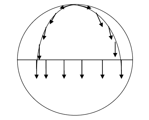
An intuitive example of curvature can be found on the surface of the Earth. Suppose we walk from the North Pole to the equator along a meridian while holding a stick horizontally. At the equator we turn 90 degrees, walk along the equator, and then return to the North Pole along a different meridian. Even though we keep the stick pointing in the “same direction” throughout the journey, it points in a different direction upon returning. This discrepancy arises from the curvature of the surface.
In a similar way, we can parallel transport a vector around an infinitesimal loop on a manifold. In flat space the vector remains unchanged; in curved space it does not. This difference under parallel transport is directly related to the Riemann tensor.
We define parallel transport as motion for which the covariant derivative of a vector vanishes. To derive the Riemann tensor, we investigate how the result of taking two covariant derivatives depends on their order. The commutator of covariant derivatives provides a measure of curvature.
2.10.1.1 Covariant Derivative Commutator
A commutator refers here to the difference between two operations, where one is performed in one order and the other in the opposite order. The commutator is defined as: \[ [A,B] = AB - BA \]
The commutator therefore vanishes only when the order of the two operations is irrelevant.
To obtain the Riemann tensor, the covariant derivative is chosen as the operation. The commutator of two covariant derivatives measures the difference between parallel transporting a tensor first in one direction and then in the opposite direction. Thus, as a measure of the difference of the tensor along the path, the covariant derivative of the tensor is used.
In flat space, the order of covariant derivatives does not matter, because covariant differentiation reduces to partial differentiation, and the commutator must therefore vanish. Conversely, any non-zero result obtained by applying the commutator to covariant differentiation can be attributed to the curvature of space, and is therefore identified as the Riemann tensor.
2.10.1.2 Derivation of the Riemann Tensor
The goal is now to derive the Riemann tensor by evaluating the following commutator: \[ \nabla_c,\nabla_b V_a = \nabla_c\nabla_b V_a - \nabla_b\nabla_c V_a \]
We know that the covariant derivative of \(V_a\) is given by (see equation 32): \[ \nabla_b V_a = \frac{\partial V_a}{\partial x^b} - \Gamma^\alpha_{b d} V_d \]
And that this derivative itself is a tensor. As we saw in the previous chapter (see equation 42): \[ T_{mn}^y = \nabla_n V_m = \frac{\partial V_m}{\partial y^n} - \Gamma^r_{n m} V_r^x \]
Thus, the covariant derivative of a vector is itself a tensor.
The covariant derivative of a tensor is given by (see equation 43): \[ \nabla_\alpha T_{\mu\nu} = \frac{\partial T_{\mu\nu}}{\partial x^\alpha} - T_{\beta\nu} \Gamma^\beta_{\alpha\mu} - T_{\mu\gamma} \Gamma^\gamma_{\alpha\nu} \]
This results in: \[ \nabla_c\nabla_b V_a = \frac{\partial}{\partial x^c} \nabla_b V_a - \Gamma^\alpha_{c e} \nabla_b V_e - \Gamma^b_{c e} \nabla_e V_a \]
After subtraction and simplification, the result can be written as:
\[ [\nabla_c, \nabla_b] V_a = R^\alpha{}_{a b c} V_\alpha \]
We now define the expression multiplying \(V_\alpha\) as the Riemann curvature tensor:
\[ R^\alpha{}_{a b c} = \frac{\partial \Gamma^\alpha_{c d}}{\partial x^b} - \frac{\partial \Gamma^\alpha_{b d}}{\partial x^c} + \Gamma^\alpha_{c e} \Gamma^b_{e d} - \Gamma^\alpha_{b e} \Gamma^c_{e d} \]
This is the component form of the Riemann curvature tensor. It explicitly contains derivatives of the Christoffel symbols and their products, demonstrating that curvature is an intrinsic geometric property that cannot be removed by any coordinate transformation.
Note: The commutator may be viewed as the difference between two vectors. The magnitude of this resulting vector is the Riemann tensor.
2.10.1.3 Alternative Derivation of the Riemann Tensor via the Commutator
In flat space the two resulting vectors coincide; in curved space they differ. This difference encodes the curvature.
2.10.1.4 Definition of the Riemann Tensor
\[ R^\gamma{}_{\mu\nu m} = \frac{\partial \Gamma^\gamma{}_{\nu m}}{\partial x^\mu} - \frac{\partial \Gamma^\gamma{}_{\mu m}}{\partial x^\nu} + \Gamma^\gamma{}_{\nu k} \Gamma^k{}_{\mu m} - \Gamma^\gamma{}_{\mu k} \Gamma^k{}_{\nu m} \]
2.10.1.5 Conclusion
This alternative derivation shows how curvature arises from the non-commutativity of covariant derivatives. The Riemann tensor is therefore a fundamental tool in general relativity, encoding the geometric and gravitational structure of spacetime.
2.10.2 Derivation of the Riemann Tensor via Geodesic Deviation
Imagine a cloud of freely falling particles. In flat spacetime, nearby geodesics remain parallel. In curved spacetime, they converge or diverge — this is geodesic deviation.
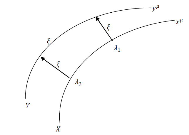
The relative acceleration between two neighboring geodesics is governed by the geodesic deviation equation: \[ \frac{D^2 \xi^\alpha}{d\tau^2} = - R^\alpha{}_{\mu\beta\nu} \, u^\mu u^\nu \, \xi^\beta \]
Here, \(u^\mu = \frac{dx^\mu}{d\tau}\) is the four-velocity of the reference particle, and \(\xi^\alpha\) is the separation vector between the two nearby geodesics.
In flat space-time the Riemann tensor vanishes, \(R^\alpha{}_{\mu\beta\nu} = 0\), and therefore the relative acceleration is zero. Neighboring geodesics remain parallel.
Since each particle follows a geodesic line, the equation of motion for their respective coordinates is given by (see equation_2_6_1):
\[ 0 = \frac{d^2 x^\alpha}{d\tau^2} + \Gamma^\alpha_{\mu\nu}(x^\alpha(\tau)) \frac{dx^\mu}{d\tau} \frac{dx^\nu}{d\tau} \] \[ 0 = \frac{d^2 y^\alpha}{d\tau^2} + \Gamma^\alpha_{\mu\nu}(y^\alpha(\tau)) \frac{dy^\mu}{d\tau} \frac{dy^\nu}{d\tau} \]
In each of these equations, the Christoffel symbols are equal at the respective particle positions \(x\) and \(y\). Since the separation between the particles is infinitesimal, we evaluate the Christoffel symbol at the position \(y^\alpha(\tau)\) by means of a Taylor series expansion:
\[ f(x) = f(a) + \frac{f'(a)}{1!}(x-a) + \frac{f''(a)}{2!}(x-a)^2 +\ldots+ \frac{f^{(n)}(a)}{n!}(x-a)^n \]
Approximating to first order only, since \(\xi\) is infinitesimal, we obtain: \[ \Gamma^\alpha_{\mu\nu}(y^\alpha(\tau)) \approx \Gamma^\alpha_{\mu\nu}(x^\alpha(\tau)) + \xi^\sigma \partial_\sigma \Gamma^\alpha_{\mu\nu}(x^\alpha(\tau)) \]
This can also be approximated as follows for an infinitesimal \(\Delta x\):
\[ \frac{d\Gamma^\alpha_{\mu\nu}(x)}{dx} = \frac{\Gamma^\alpha_{\mu\nu}(x+\Delta x)-\Gamma^\alpha_{\mu\nu}(x)}{\Delta x} \] \[ \Gamma^\alpha_{\mu\nu}(x+\Delta x) = \Gamma^\alpha_{\mu\nu}(x) + \Delta x \frac{d\Gamma^\alpha_{\mu\nu}(x)}{dx} \] \[ \Delta x=\xi \quad\Rightarrow\quad \Gamma^\alpha_{\mu\nu}(x+\xi) = \Gamma^\alpha_{\mu\nu}(x) + \xi \frac{d\Gamma^\alpha_{\mu\nu}(x)}{dx} \]
Assuming that \[ y^\alpha(\tau) = x^\alpha(\tau) + \xi^\alpha(\tau) \] and substituting this expression into the geodesic equation of particle \(y\), we obtain:
\[ 0 = \frac{d^2 y^\alpha}{d\tau^2} + \Gamma^\alpha_{\mu\nu}(y^\alpha(\tau)) \frac{dy^\mu}{d\tau} \frac{dy^\nu}{d\tau} \] \[ 0 = \frac{d^2 (x^\alpha+\xi^\alpha)}{d\tau^2} + \left( \Gamma^\alpha_{\mu\nu} + \xi^\sigma \partial_\sigma\Gamma^\alpha_{\mu\nu} \right) \left( \frac{dx^\mu}{d\tau} + \frac{d\xi^\mu}{d\tau} \right) \left( \frac{dx^\nu}{d\tau} + \frac{d\xi^\nu}{d\tau} \right) \]
Here, the Christoffel symbols and their first-order derivatives are now evaluated at \(x^\alpha(\tau)\).
Expanding all terms in the parentheses and neglecting second-order terms in \(\xi\), we obtain:
\[ 0 = \frac{d^2 x^\alpha}{d\tau^2} + \frac{d^2 \xi^\alpha}{d\tau^2} + \Gamma^\alpha_{\mu\nu} \frac{dx^\mu}{d\tau} \frac{dx^\nu}{d\tau} + \frac{dx^\mu}{d\tau} \frac{d\xi^\nu}{d\tau} + \frac{d\xi^\mu}{d\tau} \frac{dx^\nu}{d\tau} + \xi^\sigma \partial_\sigma\Gamma^\alpha_{\mu\nu} \frac{dx^\mu}{d\tau} \frac{dx^\nu}{d\tau} \]
Since the Christoffel symbols are symmetric with respect to their lower indices, these terms can be combined:
\[ 0 = \frac{d^2 x^\alpha}{d\tau^2} + \frac{d^2 \xi^\alpha}{d\tau^2} + \Gamma^\alpha_{\mu\nu} \frac{dx^\mu}{d\tau} \frac{dx^\nu}{d\tau} + 2 \frac{dx^\mu}{d\tau} \frac{d\xi^\nu}{d\tau} + \xi^\sigma \partial_\sigma\Gamma^\alpha_{\mu\nu} \frac{dx^\mu}{d\tau} \frac{dx^\nu}{d\tau} \]
Using the geodesic equation of particle \(x\) (see equation_2_6_1):
\[ \frac{d^2 x^\alpha}{d\tau^2} = - \Gamma^\alpha_{\mu\nu} \frac{dx^\mu}{d\tau} \frac{dx^\nu}{d\tau} \]
the first and third terms cancel, yielding:
\[ 0 = \frac{d^2 \xi^\alpha}{d\tau^2} + 2 \Gamma^\alpha_{\mu\nu} u^\mu \frac{d\xi^\nu}{d\tau} + \xi^\sigma \partial_\sigma\Gamma^\alpha_{\mu\nu} u^\mu u^\nu \]
or equivalently:
\[ \frac{d^2 \xi^\alpha}{d\tau^2} = - 2 \Gamma^\alpha_{\mu\nu} u^\mu \frac{d\xi^\nu}{d\tau} - \xi^\sigma \partial_\sigma\Gamma^\alpha_{\mu\nu} u^\mu u^\nu \]
Here, \[ u^\mu = \frac{dx^\mu}{d\tau} \] is the four-velocity of the reference particle.
Next, we obtain an expression for \(\dfrac{d\xi^\alpha}{d\tau}\), but this is not the total derivative of the four-vector \(\xi\), since the derivative may also receive a contribution from the change of the basis vectors while the object moves along its geodesic. To obtain the total derivative, we use:
\[ \frac{d\xi}{d\tau} = \frac{d}{d\tau}\left(\xi^\alpha \mathbf{e}_\alpha\right) = \frac{d\xi^\alpha}{d\tau}\mathbf{e}_\alpha + \xi^\alpha \frac{d\mathbf{e}_\alpha}{d\tau} = \frac{d\xi^\alpha}{d\tau}\mathbf{e}_\alpha + \xi^\alpha \frac{dx^\mu}{d\tau}\frac{d\mathbf{e}_\alpha}{dx^\mu}. \]By replacing the dummy index \(\alpha\) with \(\sigma\) in the second term and using the definition of the Christoffel symbols, we obtain:
\[ \xi^\sigma \frac{dx^\mu}{d\tau} \frac{d\mathbf{e}_\sigma}{dx^\mu} = \xi^\sigma \frac{dx^\mu}{d\tau} \Gamma^{\alpha}_{\mu\sigma}\mathbf{e}_\alpha = \xi^\sigma u^\mu \Gamma^{\alpha}_{\mu\sigma}\mathbf{e}_\alpha. \]Hence,
\[ \frac{d\xi}{d\tau} = \frac{d\xi^\alpha}{d\tau}\mathbf{e}_\alpha + \xi^\sigma u^\mu \Gamma^{\alpha}_{\mu\sigma}\mathbf{e}_\alpha = \left( \frac{d\xi^\alpha}{d\tau} + \Gamma^{\alpha}_{\mu\sigma}\xi^\sigma u^\mu \right)\mathbf{e}_\alpha, \]so that:
\[ \left(\frac{d\xi}{d\tau}\right)^\alpha = \frac{d\xi^\alpha}{d\tau} + \Gamma^{\alpha}_{\mu\sigma}\xi^\sigma u^\mu. \]Since \(\xi\) is a four-vector, its derivative with respect to proper time is also a four-vector. Therefore, we can obtain the second absolute derivative by applying the same procedure used for the first-order derivative:
\[ \frac{d}{d\tau}\left(\frac{d\xi}{d\tau}\right)^\alpha = \frac{d}{d\tau}\left(\frac{d\xi^\alpha}{d\tau}\right) + \Gamma^{\alpha}_{\mu\sigma} u^\mu \frac{d\xi^\sigma}{d\tau}. \] \[ \frac{d^2\xi^\alpha}{d\tau^2} = \frac{d^2\xi^\alpha}{d\tau^2} + \frac{d\Gamma^{\alpha}_{\mu\sigma}}{d\tau} u^\mu \xi^\sigma + \Gamma^{\alpha}_{\mu\sigma} \frac{du^\mu}{d\tau}\xi^\sigma + 2\Gamma^{\alpha}_{\mu\sigma} u^\mu \frac{d\xi^\sigma}{d\tau} + \Gamma^{\alpha}_{\mu\sigma}\Gamma^{\sigma}_{\beta\gamma} u^\mu u^\beta \xi^\gamma. \]Using the Christoffel symbols and the Taylor expansion above, and replacing \(\nu\) with \(\sigma\) in the first term, we obtain:
\[ \frac{d^2\xi^\alpha}{d\tau^2} = -2\Gamma^{\alpha}_{\mu\sigma} u^\mu \frac{d\xi^\sigma}{d\tau} - \frac{d\Gamma^{\alpha}_{\mu\nu}}{dx^\sigma} u^\mu u^\nu \xi^\sigma. \]The second term can be rewritten since the Christoffel symbols depend on \(\tau\) through the position of the reference particle:
\[ \frac{d\Gamma^{\alpha}_{\mu\sigma}}{d\tau} u^\mu \xi^\sigma = \frac{d\Gamma^{\alpha}_{\mu\sigma}}{dx^\nu} u^\nu u^\mu \xi^\sigma. \]Using the geodesic equation,
\[ \frac{d^2x^\mu}{d\tau^2} = -\Gamma^{\mu}_{\nu\gamma} u^\nu u^\gamma = \frac{du^\mu}{d\tau}, \]we find:
\[ \Gamma^{\alpha}_{\mu\sigma}\frac{du^\mu}{d\tau}\xi^\sigma = -\Gamma^{\alpha}_{\gamma\sigma}\Gamma^{\gamma}_{\nu\mu} u^\nu u^\mu \xi^\sigma. \]After relabeling dummy indices and collecting all terms, we arrive at:
\[ \frac{d^2\xi^\alpha}{d\tau^2} = -\left( \frac{d\Gamma^{\alpha}_{\mu\nu}}{dx^\sigma} - \frac{d\Gamma^{\alpha}_{\mu\sigma}}{dx^\nu} + \Gamma^{\alpha}_{\sigma\gamma}\Gamma^{\gamma}_{\nu\mu} - \Gamma^{\alpha}_{\nu\gamma}\Gamma^{\gamma}_{\mu\sigma} \right) u^\nu u^\mu \xi^\sigma. \]Since this is a tensor equation, the quantity in parentheses is itself a tensor, which allows us to define the Riemann tensor as:
\[ R^{\alpha}_{\ \mu\sigma\nu} = \frac{d\Gamma^{\alpha}_{\mu\nu}}{dx^\sigma} - \frac{d\Gamma^{\alpha}_{\mu\sigma}}{dx^\nu} + \Gamma^{\alpha}_{\sigma\gamma}\Gamma^{\gamma}_{\mu\nu} - \Gamma^{\alpha}_{\nu\gamma}\Gamma^{\gamma}_{\mu\sigma}. \]The equation can therefore be written in its compact form, known as the geodesic deviation equation:
\[ \frac{d^2\xi^\alpha}{d\tau^2} = - R^{\alpha}_{\ \mu\sigma\nu} u^\nu u^\mu \xi^\sigma. \]Since the only quantity in this equation that depends intrinsically on the metric is the Riemann tensor, we see that spacetime is flat if this tensor vanishes identically. However, if even a single component of this tensor is nonzero, spacetime is curved.
2.10.3 Key Points and Intuition
- The Riemann tensor \(R^{\sigma}_{\mu\nu\rho}\) is the fundamental tensor that describes the curvature of spacetime.
- It can be derived either from the commutator of covariant derivatives or from the geodesic deviation equation.
- Its component form is: \[ R^{\alpha}_{\ \mu\sigma\nu} = \frac{d\Gamma^{\alpha}_{\mu\nu}}{dx^\sigma} - \frac{d\Gamma^{\alpha}_{\mu\sigma}}{dx^\nu} + \Gamma^{\alpha}_{\sigma\gamma}\Gamma^{\gamma}_{\mu\nu} - \Gamma^{\alpha}_{\nu\gamma}\Gamma^{\gamma}_{\mu\sigma}. \]
- For a geodesic worldline, the following property holds: \[ 0 = \frac{d^2 x^\beta}{d\tau^2} + \Gamma^{\beta}_{\mu\nu} \frac{\partial x^\mu}{\partial \tau} \frac{\partial x^\nu}{\partial \tau}, \qquad \text{(geodesic equation)} \]
- Or equivalently: \[ \frac{d^2 x^\beta}{d\tau^2} = - \Gamma^{\beta}_{\mu\nu} u^\nu u^\mu. \]
- For the deviation between a geodesic and an infinitesimally nearby geodesic, one obtains: \[ \frac{d^2 \xi^\alpha}{d\tau^2} = - R^{\alpha}_{\ \mu\sigma\nu} u^\nu u^\mu \xi^\sigma, \qquad \text{(geodesic deviation equation)} \]
- A non-vanishing Riemann tensor implies curved spacetime and therefore the presence of gravitation.
- It measures the non-commutativity of two covariant derivatives acting on a vector: \[ \left(\nabla_\mu \nabla_\nu - \nabla_\nu \nabla_\mu\right) V^\rho = R^{\sigma}_{\mu\nu\rho} V^\sigma. \] The tensor can be fully expressed in terms of Christoffel symbols and their derivatives.
- In flat spacetime, \(R^{\sigma}_{\mu\nu\rho} = 0\); in curved spacetime, it is generally nonzero.
- Curvature is locally measurable through the behavior of geodesics: if two freely falling particles that start close together deviate from one another, this indicates curvature.
Intuitive Picture
Imagine two rockets starting side by side in space, with their engines turned off (free fall), each at a slightly different position. In flat spacetime they remain parallel, but in curved spacetime (for example near a planet) they will bend toward or away from each other.
The Riemann tensor measures exactly this effect:
- How does the “direction” of a vector change when it is transported around a closed loop?
- If the final vector differs from the original one, spacetime is curved.
This can be compared to carrying an arrow around a loop on the surface of a sphere: upon returning to the starting point, the arrow no longer points in the same direction. Curvature manifests itself as a change in direction.
Summary Table
| Quantity | Meaning |
|---|---|
| \(R^{\rho}_{\sigma\mu\nu}\) | Measures curvature via comparison of parallel transport |
| Building blocks | Christoffel symbols and their derivatives |
| Physical meaning | Deviation between nearby geodesics |
| Flat spacetime | \(R^{\rho}_{\sigma\mu\nu} = 0\) |
| Rank | Fourth-rank tensor (four indices) |
2.11 Symmetries and Independent Components
In the preceding chapters we derived the rather complex expression for the Riemann curvature tensor — a combination of derivatives and products of Christoffel symbols, with a total of 256 (=4⁴) components in a four-dimensional spacetime. In this chapter we show that the Riemann tensor in fact has only 20 independent components, and that these are completely determined by the symmetries of the tensor and the second-order derivatives of the metric.
We investigate these symmetries in a Local Inertial Frame (LIF), in which all Christoffel symbols vanish at the origin. These symmetries are, however, not restricted to this specific frame: since tensor equations are coordinate-independent, they hold in any reference frame.
2.11.1 Definition and Reformulation
The Riemann tensor is generally defined as:
\( R^{\beta}{}_{\mu\nu}{}^{\alpha} \equiv \frac{d\Gamma^{\beta}{}_{\nu}{}^{\alpha}}{dx^{\mu}} - \frac{d\Gamma^{\beta}{}_{\mu}{}^{\alpha}}{dx^{\nu}} + \Gamma^{\mu}{}_{\gamma}{}^{\alpha}\Gamma^{\beta}{}_{\nu}{}^{\gamma} - \Gamma^{\nu}{}_{\gamma}{}^{\alpha}\Gamma^{\beta}{}_{\mu}{}^{\gamma} \)
Knowing that all Christoffel symbols, \(\Gamma = 0\), vanish at the origin of the Local Inertial Frame, this reduces to:
\( R^{\beta}{}_{\mu\nu}{}^{\alpha} \equiv \frac{d\Gamma^{\beta}{}_{\nu}{}^{\alpha}}{dx^{\mu}} - \frac{d\Gamma^{\beta}{}_{\mu}{}^{\alpha}}{dx^{\nu}} \)
By applying the contraction mechanism, we can rewrite the Riemann tensor with all indices lowered:
\( R_{\alpha\beta\mu\nu} \equiv g_{\alpha\sigma} R^{\sigma}{}_{\beta\mu\nu} \equiv g_{\alpha\sigma} \left( \frac{d\Gamma^{\beta}{}_{\nu}{}^{\sigma}}{dx^{\mu}} - \frac{d\Gamma^{\beta}{}_{\mu}{}^{\sigma}}{dx^{\nu}} \right) \)
The Christoffel symbols can be expressed in terms of the metric:
\( \Gamma^{\beta}{}_{\nu}{}^{\sigma} = \frac{1}{2} g^{\sigma\gamma} \left( \frac{\partial g_{\nu\gamma}}{\partial x^{\beta}} + \frac{\partial g_{\gamma\beta}}{\partial x^{\nu}} - \frac{\partial g_{\beta\nu}}{\partial x^{\gamma}} \right) \)
Thus we may write:
\[ g_{\alpha\sigma}\frac{d\Gamma^{\beta}{}_{\nu}{}^{\sigma}}{dx^{\mu}} = \frac{1}{2} g_{\alpha\sigma} g^{\sigma\gamma} \left( \frac{\partial}{\partial x^{\mu}} \frac{\partial g_{\nu\gamma}}{\partial x^{\beta}} + \frac{\partial}{\partial x^{\mu}} \frac{\partial g_{\gamma\beta}}{\partial x^{\nu}} - \frac{\partial}{\partial x^{\mu}} \frac{\partial g_{\beta\nu}}{\partial x^{\gamma}} \right) + \]\[ + \frac{1}{2} g_{\alpha\sigma} \frac{\partial g^{\sigma\gamma}}{\partial x^{\mu}} \left( \frac{\partial g_{\nu\gamma}}{\partial x^{\beta}} + \frac{\partial g_{\gamma\beta}}{\partial x^{\nu}} - \frac{\partial g_{\beta\nu}}{\partial x^{\gamma}} \right) \tag{1} \]
The second term vanishes because the Christoffel symbols are zero at the origin of the local inertial frame, as noted above:
\[ \frac{1}{2} g_{\alpha\sigma} \frac{\partial g^{\sigma\gamma}}{\partial x^{\mu}} \left( \frac{\partial g_{\nu\gamma}}{\partial x^{\beta}} + \frac{\partial g_{\gamma\beta}}{\partial x^{\nu}} - \frac{\partial g_{\beta\nu}}{\partial x^{\gamma}} \right) = g_{\alpha\sigma}\frac{\partial g^{\sigma\gamma}}{\partial x^{\mu}} g_{\sigma\gamma} \Gamma^{\beta}{}_{\nu}{}^{\sigma} =0 \]
With this result and from equation (1) it follows:
\[ g_{\alpha\sigma}\frac{d\Gamma^{\beta}{}_{\nu}{}^{\sigma}}{dx^{\mu}} = \frac{1}{2}\delta_{\alpha}^{\gamma} \left( \frac{\partial}{\partial x^{\mu}} \frac{\partial g_{\nu\gamma}}{\partial x^{\beta}} + \frac{\partial}{\partial x^{\mu}} \frac{\partial g_{\gamma\beta}}{\partial x^{\nu}} - \frac{\partial}{\partial x^{\mu}} \frac{\partial g_{\beta\nu}}{\partial x^{\gamma}} \right) = \frac{1}{2} \left( \frac{\partial}{\partial x^{\mu}} \frac{\partial g_{\nu\alpha}}{\partial x^{\beta}} + \frac{\partial}{\partial x^{\mu}} \frac{\partial g_{\alpha\beta}}{\partial x^{\nu}} - \frac{\partial}{\partial x^{\mu}} \frac{\partial g_{\beta\nu}}{\partial x^{\alpha}} \right) \]
Interchanging the indices \(\mu\) and \(\nu\) yields the second term of the Riemann tensor expression:
\[ g_{\alpha\sigma}\frac{d\Gamma^{\beta}{}_{\mu}{}^{\sigma}}{dx^{\nu}} = \frac{1}{2} \left( \frac{\partial}{\partial x^{\nu}} \frac{\partial g_{\mu\alpha}}{\partial x^{\beta}} + \frac{\partial}{\partial x^{\nu}} \frac{\partial g_{\alpha\beta}}{\partial x^{\mu}} - \frac{\partial}{\partial x^{\nu}} \frac{\partial g_{\beta\mu}}{\partial x^{\alpha}} \right) \]
The middle terms cancel upon subtraction of the last two expressions, resulting in:
\[ R_{\alpha\beta\mu\nu} = g_{\alpha\sigma} \left( \frac{d\Gamma^{\beta}{}_{\nu}{}^{\sigma}}{dx^{\mu}} - \frac{d\Gamma^{\beta}{}_{\mu}{}^{\sigma}}{dx^{\nu}} \right) \]
\[ R_{\alpha\beta\mu\nu} = \frac{1}{2} \left( \frac{\partial}{\partial x^{\mu}} \frac{\partial g_{\nu\alpha}}{\partial x^{\beta}} + \frac{\partial}{\partial x^{\nu}} \frac{\partial g_{\beta\mu}}{\partial x^{\alpha}} - \frac{\partial}{\partial x^{\nu}} \frac{\partial g_{\mu\alpha}}{\partial x^{\beta}} - \frac{\partial}{\partial x^{\mu}} \frac{\partial g_{\beta\nu}}{\partial x^{\alpha}} \right) \tag{2} \]
Multiplying by \(-1\):
\[ R_{\alpha\beta\mu\nu} = -\frac{1}{2} \left( \frac{\partial}{\partial x^{\nu}} \frac{\partial g_{\mu\alpha}}{\partial x^{\beta}} + \frac{\partial}{\partial x^{\mu}} \frac{\partial g_{\beta\nu}}{\partial x^{\alpha}} - \frac{\partial}{\partial x^{\mu}} \frac{\partial g_{\nu\alpha}}{\partial x^{\beta}} - \frac{\partial}{\partial x^{\nu}} \frac{\partial g_{\beta\mu}}{\partial x^{\alpha}} \right) \tag{3} \]
Interchanging \(\mu\) and \(\nu\) in (2):
\[ R_{\alpha\beta\nu\mu} = \frac{1}{2} \left( \frac{\partial}{\partial x^{\nu}} \frac{\partial g_{\mu\alpha}}{\partial x^{\beta}} + \frac{\partial}{\partial x^{\mu}} \frac{\partial g_{\beta\nu}}{\partial x^{\alpha}} - \frac{\partial}{\partial x^{\mu}} \frac{\partial g_{\nu\alpha}}{\partial x^{\beta}} - \frac{\partial}{\partial x^{\nu}} \frac{\partial g_{\beta\mu}}{\partial x^{\alpha}} \right) \tag{4} \]
Thus, from (3) and (4) we obtain:
\[ R_{\alpha\beta\mu\nu} = - R_{\alpha\beta\nu\mu} \]
\[ R_{\alpha\beta\mu\nu} = - R_{\alpha\beta\nu\mu} \]
Note that this relation is only valid at the origin of the Local Inertial Frame. However, since these are tensor equations and, as we know, if tensor equations hold in one reference frame, they hold in every reference frame.
We now show in a similar manner that the Riemann tensor is antisymmetric under interchange of the first two indices:
\[ R_{\alpha\beta\mu\nu} = \frac{1}{2} \left( \frac{\partial}{\partial x^{\mu}} \frac{\partial g_{\nu\alpha}}{\partial x^{\beta}} + \frac{\partial}{\partial x^{\nu}} \frac{\partial g_{\beta\mu}}{\partial x^{\alpha}} - \frac{\partial}{\partial x^{\nu}} \frac{\partial g_{\mu\alpha}}{\partial x^{\beta}} - \frac{\partial}{\partial x^{\mu}} \frac{\partial g_{\beta\nu}}{\partial x^{\alpha}} \right) \]
\[ R_{\beta\alpha\mu\nu} = \frac{1}{2} \left( \frac{\partial}{\partial x^{\mu}} \frac{\partial g_{\nu\beta}}{\partial x^{\alpha}} + \frac{\partial}{\partial x^{\nu}} \frac{\partial g_{\alpha\mu}}{\partial x^{\beta}} - \frac{\partial}{\partial x^{\nu}} \frac{\partial g_{\mu\beta}}{\partial x^{\alpha}} - \frac{\partial}{\partial x^{\mu}} \frac{\partial g_{\alpha\nu}}{\partial x^{\beta}} \right) \]
\[ R_{\alpha\beta\mu\nu} = - R_{\beta\alpha\mu\nu} \]
If we interchange the first and third indices (\(\alpha \leftrightarrow \mu\)), and also the second and fourth (\(\beta \leftrightarrow \nu\)), we obtain:
\[ R_{\mu\nu\alpha\beta} = \frac{1}{2} \left( \frac{\partial}{\partial x^{\alpha}} \frac{\partial g_{\beta\mu}}{\partial x^{\nu}} + \frac{\partial}{\partial x^{\beta}} \frac{\partial g_{\nu\alpha}}{\partial x^{\mu}} - \frac{\partial}{\partial x^{\beta}} \frac{\partial g_{\alpha\mu}}{\partial x^{\nu}} - \frac{\partial}{\partial x^{\alpha}} \frac{\partial g_{\nu\beta}}{\partial x^{\mu}} \right) \]
\[ R_{\mu\nu\alpha\beta} = R_{\alpha\beta\mu\nu} \]
If we cyclically permute the last three indices \(\beta, \mu\), and \(\nu\), and add the three terms, we obtain:
\[ R_{\alpha\beta\mu\nu} + R_{\alpha\nu\beta\mu} + R_{\alpha\mu\nu\beta} = 0 \]
2.11.2 Symmetry Properties
From these relations, the fundamental symmetry properties of the Riemann tensor follow:
-
Antisymmetry in the last two indices:
\[ R_{\alpha\beta\mu\nu} = - R_{\alpha\beta\nu\mu} \] -
Antisymmetry in the first two indices:
\[ R_{\alpha\beta\mu\nu} = - R_{\beta\alpha\mu\nu} \] -
Symmetry under exchange of index pairs:
\[ R_{\alpha\beta\mu\nu} = R_{\mu\nu\alpha\beta} \] -
First Bianchi identity (cyclic symmetry):
\[ R_{\alpha\beta\mu\nu} + R_{\alpha\nu\beta\mu} + R_{\alpha\mu\nu\beta} = 0 \]
These antisymmetries reflect the fact that reversing the orientation of the infinitesimal loop used in parallel transport reverses the sign of the curvature contribution.
2.11.3 Number of Independent Components
In four-dimensional spacetime, a general (0,4)-tensor has \(4^4 = 256\) components. The symmetries of the Riemann tensor drastically reduce this number:
- Antisymmetry in \(\alpha\beta\) and \(\mu\nu\): reduces \(256 \rightarrow 6 \times 6 = 36\)
- Pair symmetry: \(36 \rightarrow \dfrac{6(6+1)}{2} = 21\)
- Bianchi identity: reduces further to 20 independent components
2.11.4 Key Points and Intuition
-
The Riemann tensor \( R_{\rho\sigma\mu\nu} \) possesses several symmetries:
- Antisymmetry in the last two indices:
\[ R_{\rho\sigma\mu\nu} = - R_{\rho\sigma\nu\mu} \] - Antisymmetry in the first two indices:
\[ R_{\rho\sigma\mu\nu} = - R_{\sigma\rho\mu\nu} \] - Pair symmetry:
\[ R_{\rho\sigma\mu\nu} = R_{\mu\nu\rho\sigma} \] - Bianchi identity:
\[ R_{\rho\sigma\mu\nu} + R_{\rho\mu\nu\sigma} + R_{\rho\nu\sigma\mu} = 0 \]
- Antisymmetry in the last two indices:
- Because of these symmetries, the Riemann tensor in 4D has only 20 independent components.
Thus, although the explicit expression for the Riemann tensor appears complicated, its internal structure is highly constrained. These 20 independent components encode all possible intrinsic curvature information of a four-dimensional spacetime.
Intuitive Picture
Imagine a four-index object as a cube with 256 entries. Symmetries act like mirror relations: swapping certain indices flips signs or leaves values unchanged. As with a painting that has mirror symmetry, knowing one region determines many others. The Riemann tensor works the same way: most entries are not independent.
Summary Table
| Symmetry | Meaning |
|---|---|
| \( R_{\rho\sigma\mu\nu} = - R_{\rho\sigma\nu\mu} \) | Antisymmetry in last two indices |
| \( R_{\rho\sigma\mu\nu} = - R_{\sigma\rho\mu\nu} \) | Antisymmetry in first two indices |
| \( R_{\rho\sigma\mu\nu} = R_{\mu\nu\rho\sigma} \) | Pair symmetry |
| Bianchi identity | Linear relation among cyclic permutations |
| Total in 4D | 20 independent components |
The Bianchi identity is a tensor equation that holds universally — in every coordinate system.
2.12 Bianchi Identity and Ricci Tensor
The Bianchi identity plays a crucial role in the derivation of Einstein’s field equations. Although the Riemann curvature tensor itself does not appear directly in these equations, we can derive two other important curvature quantities from it — via contraction — namely the Ricci tensor and the Ricci scalar.
In this chapter we introduce these three fundamental objects and explain their mutual relationship, beginning with the derivation of the Bianchi identity.
2.12.1 Bianchi Identity
The Bianchi identity reads: \[ \nabla_\sigma R_{\alpha\beta\mu\nu} + \nabla_\nu R_{\alpha\beta\sigma\mu} + \nabla_\mu R_{\alpha\beta\nu\sigma} = 0 \]
From the previous Chapter 2.11, Symmetries and Independent Components, we know that at the origin of a Local Inertial Frame the Riemann tensor can be written as: \[ R_{\alpha\beta\mu\nu} = \frac{1}{2} \left( \frac{\partial}{\partial x^\beta}\frac{\partial g_{\nu\alpha}}{\partial x^\mu} + \frac{\partial}{\partial x^\alpha}\frac{\partial g_{\beta\mu}}{\partial x^\nu} - \frac{\partial}{\partial x^\beta}\frac{\partial g_{\mu\alpha}}{\partial x^\nu} - \frac{\partial}{\partial x^\alpha}\frac{\partial g_{\beta\nu}}{\partial x^\mu} \right) \]
Because the Christoffel symbols vanish at the origin of this frame, the covariant derivative there reduces to the ordinary derivative: \[ \nabla_\sigma V^\alpha = \frac{\partial V^\alpha}{\partial x^\sigma} \] Thus, at the origin we have: \[ \nabla_\sigma R_{\alpha\beta\mu\nu} = \frac{\partial R_{\alpha\beta\mu\nu}}{\partial x^\sigma} \]
Substituting the expression for the Riemann tensor yields: \[ \nabla_\sigma R_{\alpha\beta\mu\nu} = \frac{\partial}{\partial x^\sigma} R_{\alpha\beta\mu\nu} = \frac{1}{2} \left( \frac{\partial}{\partial x^\sigma} \frac{\partial}{\partial x^\beta} \frac{\partial g_{\nu\alpha}}{\partial x^\mu} + \frac{\partial}{\partial x^\sigma} \frac{\partial}{\partial x^\alpha} \frac{\partial g_{\beta\mu}}{\partial x^\nu} - \frac{\partial}{\partial x^\sigma} \frac{\partial}{\partial x^\beta} \frac{\partial g_{\mu\alpha}}{\partial x^\nu} - \frac{\partial}{\partial x^\sigma} \frac{\partial}{\partial x^\alpha} \frac{\partial g_{\beta\nu}}{\partial x^\mu} \right) \]
By cyclically permuting the derivative index with the last two indices, \(\mu,\nu\), of the tensor, we obtain: \[ \nabla_\nu R_{\alpha\beta\sigma\mu} = \frac{\partial}{\partial x^\nu} R_{\alpha\beta\sigma\mu} = \frac{1}{2} \left( \frac{\partial}{\partial x^\nu} \frac{\partial}{\partial x^\beta} \frac{\partial g_{\mu\alpha}}{\partial x^\sigma} + \frac{\partial}{\partial x^\nu} \frac{\partial}{\partial x^\alpha} \frac{\partial g_{\beta\sigma}}{\partial x^\mu} - \frac{\partial}{\partial x^\nu} \frac{\partial}{\partial x^\beta} \frac{\partial g_{\alpha\sigma}}{\partial x^\mu} - \frac{\partial}{\partial x^\nu} \frac{\partial}{\partial x^\alpha} \frac{\partial g_{\beta\mu}}{\partial x^\sigma} \right) \] \[ \nabla_\mu R_{\alpha\beta\nu\sigma} = \frac{\partial}{\partial x^\mu} R_{\alpha\beta\nu\sigma} = \frac{1}{2} \left( \frac{\partial}{\partial x^\mu} \frac{\partial}{\partial x^\beta} \frac{\partial g_{\sigma\alpha}}{\partial x^\nu} + \frac{\partial}{\partial x^\mu} \frac{\partial}{\partial x^\alpha} \frac{\partial g_{\beta\nu}}{\partial x^\sigma} - \frac{\partial}{\partial x^\mu} \frac{\partial}{\partial x^\beta} \frac{\partial g_{\alpha\nu}}{\partial x^\sigma} - \frac{\partial}{\partial x^\mu} \frac{\partial}{\partial x^\alpha} \frac{\partial g_{\beta\sigma}}{\partial x^\nu} \right) \]
Adding these three equations and using the commutativity of partial derivatives, we see that the terms cancel pairwise, yielding the Bianchi identity: \[ \nabla_\sigma R_{\alpha\beta\mu\nu} + \nabla_\nu R_{\alpha\beta\sigma\mu} + \nabla_\mu R_{\alpha\beta\nu\sigma} = 0 \]
This Bianchi identity is a tensor equation that is universally valid — in every coordinate system.
2.12.2 Key Points and Intuition
-
The Bianchi identity is a fundamental structural relation satisfied by the Riemann tensor:
\[ \nabla_\lambda R^\rho{}_{\sigma\mu\nu} + \nabla_\mu R^\rho{}_{\sigma\nu\lambda} + \nabla_\nu R^\rho{}_{\sigma\lambda\mu} = 0 \] -
Contracting indices (e.g., idx with id) yields the contracted Bianchi identity:
\[ \nabla^{\mu} \left(R_{\mu\nu} - \tfrac{1}{2} g_{\mu\nu} R \right) = 0 \] - This contracted identity is essential for the internal consistency of the Einstein field equations.
-
It implies that the Einstein tensor
\[ G_{\mu\nu} = R_{\mu\nu} - \tfrac{1}{2} g_{\mu\nu} R \]
is divergence-free:
\[ \nabla^\mu G_{\mu\nu} = 0 \] - This condition corresponds physically to the conservation of energy and momentum in curved spacetime.
Intuition
The Riemann tensor is not an arbitrary object; its components must satisfy deep structural constraints. The Bianchi identity expresses one of these constraints — a built‑in consistency condition for spacetime curvature.
In vector calculus, one often encounters statements like “the divergence of a curl is zero,” reflecting structural identities. The Bianchi identity plays a similar role for curvature: certain combinations of derivatives of the Riemann tensor must always vanish. This ensures, among other things, that the Einstein equations cannot violate conservation laws.
The contracted Bianchi identity guarantees that the Einstein tensor \(G_{\mu\nu}\) automatically satisfies a conservation law, ensuring that energy and momentum are conserved in any curved spacetime.
Summary Table
| Quantity | Meaning |
|---|---|
| Bianchi identity | Structural symmetry of the Riemann tensor |
| Contracted Bianchi identity | Implies \( \nabla^\mu G_{\mu\nu} = 0 \) |
| Einstein tensor \(G_{\mu\nu}\) | \( G_{\mu\nu} = R_{\mu\nu} - \tfrac{1}{2} g_{\mu\nu} R \) |
| Physical meaning | Ensures conservation of energy–momentum in curved spacetime |
The Bianchi identity is a tensor equation that holds universally — in every coordinate system.
2.12.3 The Ricci Tensor
In the next chapter we will focus on the energy–momentum tensor. This tensor is a rank-2 tensor. For this reason, we must reduce the rank-4 Riemann tensor to a rank-2 tensor, which is called the Ricci tensor. This can be done by contracting indices, e.g., id and idx, with the metric tensor.
By contracting the first and third indices of the Riemann tensor, we obtain the Ricci tensor: \[ g^{\alpha\beta} R_{\alpha\mu\beta\nu} = R^{\beta}_{\mu\beta\nu} = R_{\mu\nu} \]
The Ricci tensor is symmetric: \[ R_{\mu\nu} = R_{\nu\mu} \]
2.12.4 The Ricci Scalar
By contracting the Ricci tensor with the metric tensor along its indices (id and idx), we obtain the Ricci scalar: \[ R = g^{\mu\nu} R_{\mu\nu} \]
This scalar curvature \(R\) is the trace of the Ricci tensor.
These tensors — the Ricci tensor and the Ricci scalar — together with the metric \(g_{\mu\nu}\), form the building blocks of Einstein’s field equations. The Bianchi identity furthermore guarantees the conservation laws that follow from these equations.
2.12.5 Key Points and Intuition
-
The Ricci tensor \(R_{\mu\nu}\) is a contraction of the Riemann tensor along indices id and idx:
\[ R_{\mu\nu} = R^{\lambda}_{\mu\lambda\nu}{} \] - It contains information about how volumes change in curved spacetime (think of stretching or contraction of bundles of geodesics).
-
The Ricci scalar \(R\) is a further contraction along the metric indices:
\[ R = g^{\mu\nu} R_{\mu\nu} \] - These quantities are coordinate-independent and form the basis of the Einstein field equations.
- While the Riemann tensor fully describes local curvature, the Ricci tensor and scalar are mainly summarized measures of curvature on larger scales.
Intuitive Interpretation
Consider a group of freely falling particles within a small volume. If that volume begins to shrink or expand as time progresses, this effect is due to the Ricci tensor.
Where the Riemann tensor tells us how curvature twists directions, the Ricci tensor tells:
- “how does curvature affect the shape of a bundle of matter or light rays?”
The Ricci scalar can be seen as a single-number summary of how “curved” spacetime is at a given point.
One could say:
- Riemann = complete picture of curvature
- Ricci tensor = effect on volumes
- Ricci scalar = total curvature summarized in a single value
Overview Table:
| Quantity | Definition | Interpretation |
|---|---|---|
| Riemann tensor | \(R^\rho{}_{\sigma\mu\nu}\) | Complete local curvature |
| Ricci tensor | \(R_{\mu\nu} = R^{\lambda}_{\mu\lambda\nu}{}\) | Volume change / summarized curvature |
| Ricci scalar | \(R = g^{\mu\nu} R_{\mu\nu}\) | Total curvature in a single number |
2.13 Energy–Momentum Tensor
The ultimate goal of general relativity is to establish a relation between the geometry of spacetime and the matter or energy that deforms it. For this purpose, a suitable mathematical object is required that describes the contents of spacetime: the energy–momentum tensor.
In special relativity it has already been shown that mass, energy, and momentum are interconnected. This relation is expressed by the well-known energy–momentum equation: \[ P^2 = m_0^2 c^2 \] \[ P^2 = \eta_{\mu\nu} P^\mu P^\nu = \frac{E^2}{c^2} - p_x^2 - p_y^2 - p_z^2 = \frac{E^2}{c^2} - p^2 \] \[ \Rightarrow m_0^2 c^2 = \frac{E^2}{c^2} - p^2 \] \[ \Rightarrow E^2 = p^2 c^2 + m_0^2 c^4 \]
This suggests that, within general relativity, not only mass but also energy and momentum contribute to the gravitational field.
In the Newtonian limit, Poisson’s equation describes the gravitational field \(\Phi\), generated by a mass density \(\rho\) (see equation 16 in Appendix 7): \[ -\vec\nabla \cdot \mathbf{\vec g} = -\vec\nabla \cdot (-\vec\nabla \Phi) = 4\pi G \rho \]
This raises the question: what is the relativistic equivalent of energy density? Is it a scalar, a vector, or something else?
2.13.1 Transformation Properties: the Example of a Dust Cloud
Consider a volume \(dx \cdot dy \cdot dz\) filled with non-interacting particles that are at rest relative to each other — a so-called dust cloud. In the rest frame S of this cloud, the energy density is: \[ \rho_0 = m_0 n_0 \] where \(m_0\) is the rest mass of a particle and \(n_0\) is the number density.
In another reference frame S’, moving with velocity \(v\) in the x-direction, the Lorentz transformation yields:
- Mass: \(m_0 \rightarrow m_0 \gamma\)
- Density: \(n_0 \rightarrow n_0 \gamma\) (due to length contraction)
- Thus: \(\rho = \rho_0 \gamma^2\)
Since \(\rho\) is not invariant, it cannot be a scalar. It is also not a component of a four-vector, because then it would transform only linearly with \(\gamma\). The \(\gamma^2\) transformation suggests that \(\rho\) behaves as a component of a rank-2 tensor — namely as the tt-component of a symmetric tensor.
2.13.2 The Energy–Momentum Tensor of Dust
The four-velocity vector of the dust cloud in S’ is: \[ u^\mu = \frac{dx^\mu}{d\tau} = \frac{dx^\mu}{dt}\frac{dt}{d\tau} = v^\mu \frac{dt}{d\tau} = v^\mu u^t \]
\[ u^\mu = \gamma (1, \vec{v}) = \begin{pmatrix} \gamma \\ v_x \gamma \\ v_y \gamma \\ v_z \gamma \end{pmatrix} = \begin{pmatrix} u^t \\ v_x u^t \\ v_y u^t \\ v_z u^t \end{pmatrix} \]
With \(u^t = \gamma\), and knowing that the energy of each particle is \(p^t = m u^t\), the total energy density becomes: \[ \rho = n p^t = n_0 u^t m u^t = n_0 m u^t u^t = \rho_0 (u^t)^2 \]
This suggests that \(\rho\) is the tt-component of a rank-2 tensor of the form: \[ T^{\mu\nu} = T^{\nu\mu} = \rho_0 u^\mu u^\nu \] This tensor is symmetric \(T^{\mu\nu} = T^{\nu\mu}\) and is called the energy–momentum tensor, also known as the stress–energy tensor for dust.
This tensor forms the link between matter/energy and the curvature of spacetime in Einstein’s field equations. In later chapters we will see how this tensor appears on the right-hand side of Einstein’s equations.
2.13.3 Physical Meaning of the Energy–Momentum Tensor
The energy-momentum tensor is a second-order tensor, which means that it contains 16 components in the form of a 4×4 matrix:
\[ T_{\mu\nu} = \begin{pmatrix} T_{tt} & T_{tx} & T_{ty} & T_{tz} \\ T_{xt} & T_{xx} & T_{xy} & T_{xz} \\ T_{yt} & T_{yx} & T_{yy} & T_{yz} \\ T_{zt} & T_{zx} & T_{zy} & T_{zz} \end{pmatrix} \]
As discussed earlier, \(T_{tt}\) represents the energy density, i.e. the density of relativistic mass. But what is the physical meaning of the remaining 15 components?
2.13.4 Time–Space Components: Energy Flow
Let us first consider the component \(T_{tx}\): \[ T_{tx} = \rho_0 u^t u^x = n_0 m u^t u^x = n_0 u^t m u^x = n_0 u^t m u^t v_x = n p^t v_x \]
We can rewrite this as: \[ T_{tx} = \frac{n A v_x dt \cdot p^t}{A dt} \]
Here, \(A v_x dt\) represents the volume of dust that moves through an area \(A\), perpendicular to the x-direction, during the time interval \(dt\). Therefore, \(T_{tx}\) is the energy flux per unit area per unit time in the x-direction.
- \(T_{ty}\): energy flow in the y-direction
- \(T_{tz}\): energy flow in the z-direction
Because the tensor is symmetric, \(T_{\mu\nu} = T_{\nu\mu}\): \[ T_{xt} = T_{tx},\quad T_{yt} = T_{ty},\quad T_{zt} = T_{tz} \]
2.13.5 Space–Space Components: Momentum Flux (Stress)
Components with both indices spatial, i.e. \(T_{kl}\) with \(k,l \in \{x,y,z\}\): \[ T_{kl} = \rho_0 u^k u^l = n_0 m u^k u^l = n_0 m u^t v_k u^l = n v_k p^l \] \[ T^{kl} = \frac{n A v_k dt \cdot p^l}{A dt} \]
Thus, \(T^{kl}\) represents the flux of the momentum component \(p^l\) in the direction \(k\):
- \(T^{xz}\): flux of z-momentum in the x-direction
- \(T^{xy}\): flux of y-momentum in the x-direction
- \(T^{zz}\): flux of z-momentum in the z-direction (pressure)
Because the tensor is symmetric: \[ T^{xz} = T^{zx},\quad T^{xy} = T^{yx},\quad T^{yz} = T^{zy} \]
2.13.6 Summary
- \(T^{tt}\) = energy density
- \(T^{ti}\) or \(T^{it}\) = energy flow in direction \(i\)
- \(T^{ij}\) = flux of momentum \(j\) in direction \(i\) (stress, pressure, shear)
2.13.7 Covariant Differentiation of the Energy-Momentum Tensor
In flat spacetime of Special Relativity: \[ 0 = \frac{\partial T^{\mu\nu}}{\partial x^\nu} = \partial^\nu T^{\mu\nu} = T^{\mu\nu}_{,\nu} \]
2.13.8 From Flat to Curved Spacetime
In general relativity, replace the partial derivative with the covariant derivative: \[ \partial_\nu \rightarrow \nabla_\nu, \quad 0 = \nabla_\nu T^{\mu\nu} = T^{\mu\nu}_{;\nu} \]
2.14 Einstein Tensor
The Poisson equation for the gravitational field in classical (Newtonian) mechanics reads as follows (see equation_appendix_5_16):
\[ -\vec \nabla \cdot \mathbf{\vec g} = -\vec \nabla \cdot (-\vec \nabla \Phi) = 4\pi G \rho \]Here, \(\Phi\) is the gravitational potential and \(\rho\) the mass density.
Our goal is now to find a relativistic generalization of this equation. As we have seen in Section 2.13.3, the classical mass density \(\rho\) is replaced in general relativity by the energy-momentum tensor \(T^{\mu\nu}\). This tensor describes not only mass, but also energy, momentum, and pressure — all forms of energy content of spacetime.
It is therefore natural to assume that Einstein’s relativistic field equation must take the form:
\[ G^{\mu\nu} = \kappa\, T^{\mu\nu} \]Here, \(G^{\mu\nu}\) is the Einstein tensor and \(\kappa\) is a constant yet to be determined. The Einstein tensor contains all information about the curvature of spacetime and plays the role of the left-hand side of the field equations.
2.14.1 Requirements for the Einstein Tensor
Based on the physical and mathematical requirements that the field equations must satisfy, the Einstein tensor \(G^{\mu\nu}\) must fulfill the following properties:
- It must vanish in flat space-time, just as \(\mathbf{\vec g} = 0\) in the absence of mass.
- It must describe space-time curvature in a way that is linearly dependent on the Riemann curvature tensor.
- It must be a symmetric rank-2 tensor, just like \(T^{\mu\nu}\).
- It must have vanishing divergence: \(\nabla_\nu G^{\mu\nu} = 0\), so that the law of conservation of energy and momentum is preserved, \(\nabla_\nu T^{\mu\nu} = 0\).
- In the Newtonian limit, it must reduce to the Poisson equation: \(\nabla^2 \Phi = 4\pi G \rho\).
In the next chapter we will derive the explicit form of the Einstein tensor that satisfies all of these conditions.
2.14.2 First Attempt Using the Ricci Tensor as a Solution
As we saw in Chapter 2.8, the gravitational potential \(\Phi\) is related to the 00-component of the metric via: \[ \frac{d^2 \vec r}{dt^2} = -\vec \nabla \Phi =-\vec {\text{grad}}\, \Phi \quad\text{with}\quad \Phi = c^2 h_{00}/2 \tag{1} \]
It therefore seems natural to search for a tensor that—like the Laplacian—contains second derivatives of the metric. The Riemann tensor satisfies this requirement and is moreover the only known tensor that fundamentally describes space-time curvature.
Since we require a rank-2 tensor (as demanded by the Einstein field equations), it is reasonable to first consider the contracted form of the Riemann tensor: the Ricci tensor. We recall: \[ R^{\alpha}_{\mu\sigma\nu} = \frac{d\Gamma^{\alpha}_{\mu\nu}}{dx^{\sigma}} - \frac{d\Gamma^{\alpha}_{\mu\sigma}}{dx^{\nu}} + \Gamma^{\alpha}_{\sigma\gamma}\Gamma^{\gamma}_{\mu\nu} - \Gamma^{\alpha}_{\nu\gamma}\Gamma^{\gamma}_{\mu\sigma} \tag{2} \]
Contracting the upper and third index yields the Ricci tensor: \[ R_{\mu\nu} = R_{\mu\alpha\nu}^{\alpha} \tag{3} \] \[ R_{\mu\nu} = R_{\mu\alpha\nu}^{\alpha} = \frac{d\Gamma^{\alpha}_{\mu\nu}}{dx^{\alpha}} - \frac{d\Gamma^{\alpha}_{\mu\alpha}}{dx^{\nu}} + \Gamma^{\alpha}_{\alpha\gamma}\Gamma^{\gamma}_{\mu\nu} - \Gamma^{\alpha}_{\nu\gamma}\Gamma^{\gamma}_{\mu\alpha}{} \tag{4} \]
In the Newtonian limit, for a weak and static gravitational field, only one term contributes to \(R_{00}\). We find: \[ R_{00} = R^{\alpha}_{00\alpha} = \Gamma^{\alpha}_{00,\alpha} - \Gamma^{\alpha}_{0\alpha,0} + \mathcal{O}(h^2) = \Gamma^{i}{}_{00,i} \]
Since we restrict ourselves to a static field, the time derivative vanishes, leaving: \[ R_{00} = \Gamma^{i}{}_{00,i} \]
Using the previously derived expression for the Christoffel symbol in this approximation: \[ \Gamma^{i}_{00} = -\tfrac{1}{2} g^{ij} g_{00,j} \approx \tfrac{1}{2}\partial_i h_{00} \]
With the approximation \(g^{ij} = \eta^{ij}\) and \(g_{00,j} = h_{00,j}\), we obtain: \[ \Gamma^{i}_{00} = -\tfrac{1}{2}\eta^{ij}\, h_{00,j} = \tfrac{1}{2}\delta^{i}_{j}\,h_{00,j}, \qquad \Gamma^{i}_{00,i} = \tfrac{1}{2}\delta^{i}_{j}\, h_{00,ij} = \tfrac{1}{2}\, h_{00,ii} \]
\[ R_{00} = \Gamma^{i}_{0o,i} = \tfrac{1}{2} \left( \partial_1^2 h_{00} + \partial_2^2 h_{00} + \partial_3^2 h_{00} \right) \]
Substituting \(h_{00} = 2\Phi/c^2\) yields: \[ R_{00} = \tfrac{1}{2}\nabla^2 h_{00} = \frac{1}{c^2}\nabla^2 \Phi \] and therefore: \[ R_{00} = \frac{4\pi G}{c^2}\rho \]
This result suggests that a field equation of the form: \[ R_{\mu\nu} = \kappa T_{\mu\nu} \] could satisfy the Newtonian limit, with \(\kappa = 8\pi G / c^4\) as a candidate constant.
Einstein was indeed initially convinced of this equation in 1915. Using it, he even solved the
long-standing problem of the perihelion precession of Mercury. In a letter he wrote
enthusiastically:
“A few days I was beside myself with joyful excitement.”
Nevertheless, he ultimately had to abandon this first attempt. The reason was that the Ricci tensor does not, in general, have vanishing divergence, whereas the energy-momentum tensor \(T_{\mu\nu}\) does satisfy \(\nabla^\nu T_{\mu\nu} = 0\). As a result, this form could not fulfill the required conservation of energy and momentum.
2.14.3 Second Attempt
There exists a tensor closely related to the Ricci tensor that is suitable as the left-hand side of the Einstein field equations: the Einstein tensor. It is defined as: \[ G^{\mu\nu} = R^{\mu\nu} - \tfrac{1}{2} R\, g^{\mu\nu} \] where \(R = R^{a}{}_{a}\) is the Ricci scalar, i.e. the scalar curvature.
This tensor already satisfies several requirements:
- It is symmetric, as required by the symmetry of \(T^{\mu\nu}\).
- It is of rank 2.
- It describes space-time curvature, since it is constructed directly from the Ricci tensor and thus indirectly from the Riemann tensor.
What remains to be shown is that the covariant divergence of the Einstein tensor vanishes: \[ \nabla_\nu G^{\mu\nu} = 0 \] This is essential, because only then can it be consistently coupled to the energy-momentum tensor \(T^{\mu\nu}\), for which \(\nabla_\nu T^{\mu\nu} = 0\) also holds (see Chapter 2.13.2 and Chapter 2.5.2, Equation 15).
We derive this result using the Bianchi identity: \[ \nabla_\sigma R_{\alpha\beta\mu\nu} + \nabla_\nu R_{\alpha\beta\sigma\mu} + \nabla_\mu R_{\alpha\beta\nu\sigma} = 0 \]
We multiply this identity by the metric factors \(g^{\gamma\sigma} g^{\alpha\mu} g^{\beta\nu}\). Since derivatives of the metric vanish in a locally inertial frame, these factors may be brought inside: \[ \nabla_\sigma \bigl( g^{\gamma\sigma} g^{\alpha\mu} g^{\beta\nu} R_{\alpha\beta\mu\nu} \bigr) + \nabla_\nu \bigl( g^{\gamma\sigma} g^{\alpha\mu} g^{\beta\nu} R_{\alpha\beta\sigma\mu} \bigr) + \nabla_\mu \bigl( g^{\gamma\sigma} g^{\alpha\mu} g^{\beta\nu} R_{\alpha\beta\nu\sigma} \bigr) = 0 \]
The first term becomes: \[ \nabla_\sigma \bigl(g^{\gamma\sigma} R\bigr) \] where \(R = g^{\alpha\mu} g^{\beta\nu} R_{\alpha\beta\mu\nu}\) is the Ricci scalar.
For the second and third terms we use the definition of the Ricci tensor and the symmetry properties of the Riemann tensor: \[ \nabla_\nu \bigl( g^{\gamma\sigma} g^{\alpha\mu} g^{\beta\nu} R_{\alpha\beta\sigma\mu} \bigr) = -\,\nabla_\nu \bigl( g^{\gamma\sigma} g^{\beta\nu} R_{\sigma\beta} \bigr) = -\,\nabla_\nu R^{\gamma\nu} \] \[ \nabla_\mu \bigl( g^{\gamma\sigma} g^{\alpha\mu} g^{\beta\nu} R_{\alpha\beta\nu\sigma} \bigr) = -\,\nabla_\mu \bigl( g^{\gamma\sigma} g^{\alpha\mu} R_{\sigma\alpha} \bigr) = -\,\nabla_\mu R^{\gamma\mu} \]
Thus: \[ \nabla_\sigma \bigl(g^{\gamma\sigma} R\bigr) - \nabla_\nu R^{\gamma\nu} - \nabla_\mu R^{\gamma\mu} = 0 \]
Since dummy indices may be exchanged, we write: \[ \nabla_\sigma \bigl(g^{\gamma\sigma} R\bigr) - 2 \nabla_\sigma R^{\gamma\sigma} = 0 \] or: \[ \nabla_\sigma \bigl( 2 R^{\gamma\sigma} - g^{\gamma\sigma} R \bigr) = 0 \]
This can be rewritten as: \[ \nabla_\sigma \bigl( R^{\gamma\sigma} - \tfrac{1}{2} g^{\gamma\sigma} R \bigr) = 0 \] that is: \[ \nabla_\nu G^{\mu\nu} = 0 \]
2.14.4 Conclusion
The Einstein tensor \(G^{\mu\nu}\) is the appropriate choice for the left-hand side of the field equation. It is symmetric, constructed from space-time curvature, and satisfies conservation of energy and momentum through its vanishing divergence. Consequently, the equation \[ G^{\mu\nu} = \kappa T^{\mu\nu} \] is a solid candidate for the general relativistic generalization of the laws of gravitation.
2.15 Einstein Field Equations
In the previous two chapters, we derived the two quantities that form the core of the field equations in general relativity:
- The Einstein tensor \(G^{\mu\nu}\), which describes space-time curvature, and
- The energy-momentum tensor \(T^{\mu\nu}\), which represents the matter–energy content of space-time.
These two quantities are coupled in the form: \[ G^{\mu\nu} = \kappa T^{\mu\nu} \] where \(\kappa\) is a constant yet to be determined.
2.15.1 Objective: recovery of Newtonian gravity in the weak-field limit
To determine the value of \(\kappa\), we require that this equation reduces, in the Newtonian limit (weak, static fields and low velocities), to Newton’s classical law of gravitation. This ensures that general relativity is consistent with classical theories within their domain of validity.
2.15.2 Alternative formulation of the field equation
Einstein also expressed the field equations in an alternative, equivalent form. This reads: \[ G_{im} = -\chi \left(T_{im} - \tfrac{1}{2} g_{im} T\right) \tag{2a} \] where:
- \(\chi\) is a constant (related to \(\kappa\)),
- \(T = T^{\sigma}_{\sigma}\) is the trace of the energy-momentum tensor \(T_{\mu\nu}\), i.e. its contraction,
- and the right-hand side as a whole again forms a rank-2 tensor.
This formulation was used by Einstein in his famous paper “Die Feldgleichungen der Gravitation”, submitted on 25 November 1915 to the Königlich Preußische Akademie der Wissenschaften. There he writes:
“Ist in dem betrachteten Raume ‘Materie’ vorhanden, so tritt deren Energietensor auf der rechten Seite von (2) [...] auf. Wir setzen \[ G_{im} = -\chi T_{im} - \tfrac{1}{2} g_{im} T \] T ist der Skalar des Energietensors der ‘Materie’, die rechte Seite von (2) ein Tensor.”
2.15.2.1 Summary
The full form of Einstein’s field equations therefore reads: \[ R_{\mu\nu} - \tfrac{1}{2} g_{\mu\nu} R = \kappa T_{\mu\nu} \] Or equivalently: \[ G_{\mu\nu} = -\chi \left( T_{\mu\nu} - \tfrac{1}{2} g_{\mu\nu} T\right) \] In the next section, we will determine the constant \(\kappa\) by applying the equation to the Newtonian limit. This will allow us to establish the connection with classical gravitation and thus fix general relativity in its final form.
2.15.2.2 The alternative form of Einstein’s equation
We start from the standard form of the field equation: \[ R_{\mu\nu} - \tfrac{1}{2} g_{\mu\nu} R = \kappa T_{\mu\nu} \] By multiplying both sides of this equation by \(g^{\mu\nu}\), we obtain: \[ g^{\mu\nu} R_{\mu\nu} - \tfrac{1}{2} g^{\mu\nu} g_{\mu\nu} R = \kappa g^{\mu\nu} T_{\mu\nu} \] According to the definitions of contraction, we have: \[ g^{\mu\nu} R_{\mu\nu} = R \quad\text{and}\quad g^{\mu\nu} T_{\mu\nu} = T \] Thus, the equation becomes: \[ R - \tfrac{1}{2} R \cdot g^{\mu\nu} g_{\mu\nu} = \kappa T \] Since \(g^{\mu\nu}\) is the inverse of \(g_{\mu\nu}\), their product is the Kronecker delta \(\delta^{\nu}{}_{\mu}\). Contracting this tensor (i.e. summing over the diagonal elements), we obtain: \[ g^{\mu\nu} g_{\mu\nu} = \delta^{\nu}{}_{\nu} = 1 + 1 + 1 + 1 = 4 \] The equation then reduces to: \[ R - \tfrac{1}{2} R \times 4 = \kappa T \quad\Rightarrow\quad R - 2R = \kappa T \quad\Rightarrow\quad R = -\kappa T \] We can now substitute this expression for \(R\) back into the original Einstein equation: \[ R_{\mu\nu} - \tfrac{1}{2} g_{\mu\nu} \times (-\kappa T) = \kappa T_{\mu\nu} \] which leads to: \[ R_{\mu\nu} + \tfrac{1}{2} \kappa g_{\mu\nu} T = \kappa T_{\mu\nu} \quad\Rightarrow\quad R_{\mu\nu} = \kappa \left(T_{\mu\nu} - \tfrac{1}{2} g_{\mu\nu} T\right) \] We may then rewrite this by multiplying both sides by \(g^{\alpha\mu} g^{\beta\nu}\): \[ g^{\alpha\mu} g^{\beta\nu} R_{\mu\nu} = g^{\alpha\mu} g^{\beta\nu} \left( \kappa T_{\mu\nu} - \tfrac{1}{2} \kappa g_{\mu\nu} T \right) \quad\Rightarrow\quad R^{\alpha\beta} = \kappa T^{\alpha\beta} - \tfrac{1}{2} \kappa g^{\alpha\beta} T \] Replacing the indices by \(\mu\nu\), we obtain the alternative form: \[ R_{\mu\nu} = \kappa T_{\mu\nu} - \tfrac{1}{2} \kappa g_{\mu\nu} T \] Since earlier we found \(R = -\kappa T\), we may also write: \[ R_{\mu\nu} = \kappa T_{\mu\nu} + \tfrac{1}{2} g_{\mu\nu} R \] which results in: \[ R_{\mu\nu} - \tfrac{1}{2} g_{\mu\nu} R = \kappa T_{\mu\nu} \]
2.15.2.3 Conclusion
The standard form and the alternative form of Einstein’s equations are fully equivalent. They emphasize different aspects: one highlights the role of the Einstein tensor \(G_{\mu\nu} = R_{\mu\nu} - \tfrac{1}{2} g_{\mu\nu} R\), while the other emphasizes the decomposition in terms of \(R_{\mu\nu}\), \(g_{\mu\nu}\), and the trace \(T\).
This derivation confirms the consistency of Einstein’s field equations and their equivalence to the alternative formulation presented in his original publication. Both forms lead to the same physical predictions, although the alternative notation is often preferred due to its symmetry and simplicity in applications.
2.15.3 Newtonian limit
In the previous chapter, we already saw that in the limit of weak fields and low velocities, the \(R_{00}\) component of the Riemann tensor can be approximated as: \[ R_{00} \approx \frac{1}{c^{2}} \nabla^{2} \Phi \] Moreover, when the metric \(g_{\mu\nu}\) is reduced to the Minkowski metric \(\eta_{\mu\nu}\) of flat space-time, we may approximate the Ricci tensor component as: \[ R_{\mu\nu} \equiv g_{0\mu} g_{0\nu} R^{\mu\nu} \approx \eta_{0\mu} \eta_{0\nu} R^{\mu\nu} = (-1)(-1) R_{00} = R_{00} \] Combined, this yields: \[ R_{00} \approx \frac{1}{c^{2}} \nabla^{2} \Phi = \frac{4\pi G}{c^{2}} \rho \]
In this Newtonian limit, the only non-negligible component of the energy-momentum tensor \(T_{\mu\nu}\) is \(T_{00} = \rho c^{2}\). This follows from the expression: \[ T_{\mu\nu} = \rho u_{\mu} u_{\nu} \quad\text{with}\quad u_{i} \ll u_{0} = c \] We can then approximate the trace of the tensor as: \[ T = g^{\mu\nu} T_{\mu\nu} \approx g^{00} T_{00} \approx \eta^{00} T_{00} = T_{00} = \rho c^{2} \]
We now apply the 00-component of the Einstein equation: \[ R_{00} = \kappa \left(T_{00} - \tfrac{1}{2} \eta_{00} T\right) \] Substitution yields: \[ \frac{4\pi G}{c^{2}} \rho = \kappa \left(\rho c^{2} - \tfrac{1}{2}\cdot 1 \cdot \rho c^{2}\right) \quad\Rightarrow\quad \frac{4\pi G}{c^{2}} \rho = \frac{1}{2} \kappa \rho c^{2} \] From this we obtain: \[ \kappa = \frac{8\pi G}{c^{4}} \]
We can now formulate Einstein’s field equations in both their standard and alternative forms: \[ R_{\mu\nu} - \tfrac{1}{2} g_{\mu\nu} R = \frac{8\pi G}{c^{4}} T_{\mu\nu} \] Or: \[ R_{\mu\nu} = \frac{8\pi G}{c^{4}} \left( T_{\mu\nu} - \tfrac{1}{2} g_{\mu\nu} T \right) \] And in lowered-index notation (same form): \[ R_{\mu\nu} - \tfrac{1}{2} g_{\mu\nu} R = \frac{8\pi G}{c^{4}} T_{\mu\nu} \] or: \[ R_{\mu\nu} = \frac{8\pi G}{c^{4}} \left( T_{\mu\nu} - \tfrac{1}{2} g_{\mu\nu} T \right) \]
2.15.3.1 Remark 1:
The constant \(\kappa = \dfrac{8\pi G}{c^{4}}\) has an extremely small value: \[ \kappa = \frac{8\pi G}{c^{4}} \approx 2.071 \times 10^{-43}\ \text{s}^{2}\,\text{m}^{-1}\,\text{kg}^{-1} \] This means that space-time is extraordinarily “stiff”: only enormous amounts of mass or energy produce noticeable curvature.
2.15.3.2 Remark 2:
Despite the relatively simple appearance of the Einstein equations, they are in fact extremely complex. For a given distribution of matter and energy (in the form of \(T_{\mu\nu}\)), the equations form a system of ten coupled, nonlinear, second‑order partial differential equations for the metric \(g_{\mu\nu}\). These ten equations correspond to the ten independent components of the symmetric metric.
2.15.3.3 Remark 3:
The nonlinearity of the Einstein equations has deep physical meaning. It reflects the self‑referential character of gravity: space‑time influences matter and energy, but is simultaneously influenced by that same matter and energy. As Kevin Brown notes in Reflection on Relativity:
“The self‑referential nature of the metric field equations is also reflected in their nonlinearity. This is unavoidable for a theory in which the metric relations between entities determine their ‘positions’, and those positions in turn influence the metric.”
The nonlinearity also implies the possibility of interaction between gravitational fields themselves (such as via graviton exchange), something that is not possible for photons in the linear Maxwell formalism of electromagnetism.
2.15.3.4 Remark 4:
The Einstein equations impose only six independent constraints on the ten components of the metric \(g_{\mu\nu}\). The remaining four degrees of freedom are related to coordinate freedom: we may specify four arbitrary functions through the coordinates \(x^{\alpha}(P)\). This overdetermination is a direct consequence of the fact that the Einstein tensor \(G_{\mu\nu}\) has zero divergence: \(\nabla_{\mu} G^{\mu\nu} = 0\).
2.15.4 Key Points and Intuition
- The Einstein field equations couple space‑time curvature to energy‑momentum content: \[ R_{\mu\nu} - \tfrac{1}{2} g_{\mu\nu} R = \kappa T_{\mu\nu} \]
- The left-hand side, \(G_{\mu\nu} = R_{\mu\nu} - \tfrac{1}{2} g_{\mu\nu} R = \kappa T_{\mu\nu}\), is the Einstein tensor, which encodes geometry.
- The right-hand side contains the energy‑momentum tensor \(T_{\mu\nu}\), describing mass, energy, pressure, and fluxes.
- The constant \(\kappa\) is derived by matching the equations to Newton’s gravitational law in the weak‑field limit: \[ \kappa = \frac{8\pi G}{c^{4}} \]
- An alternative, fully equivalent formulation of the field equation is: \[ R_{\mu\nu} = \kappa \left( T_{\mu\nu} - \tfrac{1}{2} g_{\mu\nu} T \right) \] where \(T = g^{\mu\nu} T_{\mu\nu}\) is the trace of the energy‑momentum tensor.
- Contracting both sides of the standard form yields \(R = -\kappa T\), consistent with the alternative formulation.
Intuition
Imagine space‑time as a flexible yet stiff four‑dimensional fabric. The Einstein equations describe how that fabric is deformed by the presence of mass and energy. Like a mattress dented by a heavy ball, space‑time curves around masses. But instead of a push or force, this deformation is a geometric effect that determines how objects move—even when they “freely” fall.
The equation \(G_{\mu\nu} = \kappa T_{\mu\nu}\) then says:
- Whatever exists in space‑time (matter, energy, radiation),
- determines what space‑time itself looks like (curves, stretches, twists).
In weak fields and at low speeds, this automatically reduces to Newton’s classical gravitational equation—a crucial test for any relativistic theory.
2.15.5 Table: Important Quantities in the Einstein Field Equations
| Quantity | Meaning / Role |
|---|---|
| \(R_{\mu\nu}\) | Ricci tensor: summarized curvature |
| \(R\) | Ricci scalar: total curvature |
| \(g_{\mu\nu}\) | Metric: measurement structure of space‑time |
| \(G_{\mu\nu} = R_{\mu\nu} - \frac{1}{2} g_{\mu\nu} R\) | Einstein tensor: measures geometric deformation |
| \(T_{\mu\nu}\) | Energy‑momentum tensor: distribution of energy and matter |
| \(T = g^{\mu\nu} T_{\mu\nu}\) | Trace of \(T_{\mu\nu}\): scalar energy density |
| \(\kappa = \frac{8\pi G}{c^4}\) | Coupling constant between geometry and physics |
2.16 Summary of the Final Formula for General Relativity
In the preceding chapters we have step by step derived the Einstein field equations (EFE). Along the way we introduced all necessary building blocks, such as the Riemann tensor, the Ricci tensor, the Ricci scalar, the energy‑momentum tensor, and the use of covariant derivatives. In this concluding chapter we summarize the final result and clarify its physical meaning.
2.16.1 Einstein’s Fundamental Insight
Einstein’s central idea was that gravity is not a force in the classical sense, but the result of the curvature of space‑time. This curvature is caused by the presence of mass and energy. His goal was to find a mathematical formula describing this relationship: how mass and energy influence the geometry of space‑time.
The general form of the field equation:
Without repeating the full derivation, we present here the final result of Einstein’s theory: \[ R_{\mu\nu} - \frac{1}{2} g_{\mu\nu} R + \lambda g_{\mu\nu} = \frac{8\pi G}{c^4} T_{\mu\nu} \tag{4} \] The term \(\lambda g_{\mu\nu}\) contains the so‑called cosmological constant (\(\lambda = 1.1056 \times 10^{-52} \, \text{m}^{-2}\)), which becomes relevant only on cosmological scales. For most applications in astrophysics and classical relativity we may neglect this term, so the equation simplifies to: \[ R_{\mu\nu} - \frac{1}{2} g_{\mu\nu} R = \frac{8\pi G}{c^4} T_{\mu\nu} \tag{5} \]
The left-hand side describes the geometry (curvature) of space‑time, while the right-hand side represents the content of space (mass, energy, and momentum). In this equation, \(c\) is the speed of light (\(2.99792458 \times 10^8 \, \text{m/s}\)) and \(G\) is the gravitational constant (\(6.674 \times 10^{-11} \, \text{m}^3\text{kg}^{-1}\text{s}^{-2}\)).
2.16.2 Vacuum: outside a mass
In a region without mass or energy, \(T_{\mu\nu} = 0\). The field equation then reduces to: \[ R_{\mu\nu} - \frac{1}{2} g_{\mu\nu} R = 0 \tag{6} \] As discussed in Section 2.15.2.2 The Alternative Form of Einstein’s Equation, in that case: \[ R = -\frac{8\pi G}{c^4} T = 0 \quad\Rightarrow\quad R = 0 \] So what remains is: \[ R_{\mu\nu} = 0 \tag{7} \] These are the so‑called vacuum equations of Einstein.
2.16.3 Explanation of the Objects Used
The indices \(\mu\) and \(\nu\) run from 0 to 3 and refer to the four dimensions of space‑time: time (0) and space (1 = x, 2 = y, 3 = z). Equation (5) therefore contains 16 component equations:
\[ \begin{align*} R_{00} - \frac{1}{2} g_{00} R &= \frac{8\pi G}{c^4} T_{00}, \\ R_{01} - \frac{1}{2} g_{01} R &= \frac{8\pi G}{c^4} T_{01}, \\ &\vdots \\ R_{33} - \frac{1}{2} g_{33} R &= \frac{8\pi G}{c^4} T_{33} \end{align*} \] By symmetry (namely \(R_{\mu\nu} = R_{\nu\mu}\)) only 10 are independent.
The Ricci tensor \(R_{\mu\nu}\) is often written in matrix form as: \[ R_{\mu\nu} = \begin{pmatrix} R_{00} & R_{01} & R_{02} & R_{03} \\ R_{10} & R_{11} & R_{12} & R_{13} \\ R_{20} & R_{21} & R_{22} & R_{23} \\ R_{30} & R_{31} & R_{32} & R_{33} \end{pmatrix} \]
The metric tensor \(g_{\mu\nu}\), which contains the geometric structure of space-time, also has 10 independent components and fully determines the space-time geometry: \[ g_{\mu\nu} = \begin{pmatrix} g_{00} & g_{01} & g_{02} & g_{03} \\ g_{10} & g_{11} & g_{12} & g_{13} \\ g_{20} & g_{21} & g_{22} & g_{23} \\ g_{30} & g_{31} & g_{32} & g_{33} \end{pmatrix} \]
The Ricci scalar \(R\) follows from the contraction of the Ricci tensor with the inverse metric: \(R = g^{\mu\nu} R_{\mu\nu}\). All elements on the left-hand side of equation (5) describe the geometry of the considered space-time. On the right-hand side we find the energy-momentum tensor \(T_{\mu\nu}\), which contains all information about matter and energy in the system: \[ T_{\mu\nu} = \begin{pmatrix} T_{00} & T_{01} & T_{02} & T_{03} \\ T_{10} & T_{11} & T_{12} & T_{13} \\ T_{20} & T_{21} & T_{22} & T_{23} \\ T_{30} & T_{31} & T_{32} & T_{33} \end{pmatrix} \] Here, \(T_{00}\) represents the energy density, \(T_{0i}\) the energy flux, and \(T_{ij}\) the momentum flow and pressure components.
2.16.4 Determining \(R_{\mu\nu}\)
The Ricci tensor is computed via contraction of the Riemann tensor: \[ R_{\mu\nu} = R^{\rho}_{\mu\rho\nu} \] \[ R_{\mu\nu} = R^{\rho}_{\mu\rho\nu} = \frac{\partial \Gamma^{\rho}_{\mu\nu}}{\partial x^{\rho}} - \frac{\partial \Gamma^{\rho}_{\rho\mu}}{\partial x^{\nu}} + \Gamma^{\rho}_{\rho\lambda} \Gamma^{\lambda}_{\nu\mu} - \Gamma^{\rho}_{\nu\lambda} \Gamma^{\lambda}_{\rho\mu} \quad\text{(note 1)} \] This tensor depends on the Christoffel symbols, which themselves consist of derivatives of the metric: \[ \Gamma^{\rho}_{\mu\nu} = \frac{1}{2} g^{\rho\alpha} \left( \frac{\partial g_{\nu\alpha}}{\partial x^{\mu}} + \frac{\partial g_{\mu\alpha}}{\partial x^{\nu}} - \frac{\partial g_{\mu\nu}}{\partial x^{\alpha}} \right) \quad\text{(note 1)} \] From this it follows that the full geometry (and thus also gravity) depends on the metric \(g_{\mu\nu}\) and its derivatives.
2.16.5 The Schwarzschild Solution
In 1915 Karl Schwarzschild found an exact solution of the field equations in vacuum around a spherically symmetric mass. This led to the well-known Schwarzschild metric (see chapter 3): \[ ds^{2} = \left(1 - \frac{2GM}{c^{2}r}\right) c^{2} dt^{2} - \left(1 - \frac{2GM}{c^{2}r}\right)^{-1} dr^{2} - r^{2} d\theta^{2} - r^{2} \sin^{2}\theta d\phi^{2} \] This metric applies outside the mass, i.e. in a region where \(T_{\mu\nu} = 0\) and therefore: \(R_{\mu\nu} = 0\).
The Schwarzschild solution is particularly important because it yields experimentally verifiable predictions, such as the bending of light and the perihelion precession of Mercury. The metric tensor then consists of the elements: \[ g_{00} = 1 - \frac{2GM}{c^{2}r}, \quad g_{11} = -\left(1 - \frac{2GM}{c^{2}r}\right)^{-1}, \quad g_{22} = -r^{2}, \quad g_{33} = -r^{2} \sin^{2}\theta \] This is the so‑called trace of the tensor. Or in tensor form: \[ g_{\mu\nu} = \begin{pmatrix} 1 - \frac{2GM}{c^{2}r} & 0 & 0 & 0 \\ 0 & -\left(1 - \frac{2GM}{c^{2}r}\right)^{-1} & 0 & 0 \\ 0 & 0 & -r^{2} & 0 \\ 0 & 0 & 0 & -r^{2} \sin^{2}\theta \end{pmatrix} \]
Because the Schwarzschild equation is used outside a mass, the right-hand side of the Einstein field equations becomes zero (\(T_{\mu\nu} = 0\)). Thus the field equations reduce to equation (6), and since \(R\) is derived from \(R_{\mu\nu}\), equation (6) can only be zero when \(R_{\mu\nu} = 0\). Therefore the only relevant equation is \(R_{\mu\nu} = 0\). As mentioned earlier, the tensor \(R_{\mu\nu}\) is built from Christoffel symbols and their derivatives. All relevant Christoffel symbols for this metric have been derived and summarized in Appendix 1.2.
The Schwarzschild equation uses the polar or spherical coordinate system to describe the full space-time; however, due to conservation of angular momentum, physical motion takes place in a single plane. By choosing the appropriate polar coordinate system, this plane can be rotated so that the equatorial plane coincides with the surface under study. In that case the angle \(\theta = \pi/2\), and the metric tensor simplifies to: \[ g_{\mu\nu} = \begin{pmatrix} 1 - \frac{2GM}{c^{2}r} & 0 & 0 & 0 \\ 0 & -\left(1 - \frac{2GM}{c^{2}r}\right)^{-1} & 0 & 0 \\ 0 & 0 & -r^{2} & 0 \\ 0 & 0 & 0 & -r^{2} \end{pmatrix} \] (See also chapter 7.3 “Answers to questions concerning Schwarzschild”)
2.16.5.1 Note 1
In his document Einstein uses the opposite sign for the Christoffel symbol \(\Gamma^{\rho}_{\mu\nu}\), and the Ricci tensor \(R_{\mu\nu}\) also has the opposite sign for the third and fourth terms on the right-hand side of the equation. For the metric we have used the so‑called (+ − − −) notation, also known as the West Coast convention.
2.16.5.2 Final Remark
The Einstein field equations form a powerful system of 10 coupled, non-linear partial differential equations. Although they can be written compactly, they are rich and complex in content. They form the starting point for searching for solutions (such as the Schwarzschild solution, cosmological models) and explain a wide range of physical phenomena — from Mercury’s orbit to the expansion of the universe.
"Mass and energy determine the curvature of space-time, and the curvature of space-time determines the motion of mass and energy."
2.16.6 Key Points and Intuition
- Einstein’s central insight: gravity is not a force, but the result of the curvature of space-time caused by mass and energy.
- The Einstein field equations form the foundation of general relativity: \[ R_{\mu\nu} - \frac{1}{2} g_{\mu\nu} R + \lambda g_{\mu\nu} = \frac{8\pi G}{c^4} T_{\mu\nu} \] For most practical applications the cosmological constant \(\lambda \approx 1.1 \times 10^{-52} \, \text{m}^{-2}\) is neglected. The equation then reduces to: \[ R_{\mu\nu} - \frac{1}{2} g_{\mu\nu} R = \frac{8\pi G}{c^4} T_{\mu\nu} \]
- In vacuum (outside matter): \(T_{\mu\nu} = 0\), so: \(R_{\mu\nu} = 0\). These are the vacuum equations, which lead among other things to the Schwarzschild solution.
- Every term on the left-hand side is purely geometric (derived from the metric \(g_{\mu\nu}\)); the right-hand side contains physical information (energy, mass, pressure).
Intuitive Picture
Imagine a four-dimensional elastic fabric. Matter and energy pull on that fabric and cause deformation. That deformation determines how objects move — they follow the curvature of space-time.
The equation says:
- Left: “how is space-time curved?”
- Right: “what is in space-time that causes that curvature?”
For example:
- A planet does not move because it is “pulled” by a force,
- but because it follows a geodesic in curved space-time.
The equations are elegant and powerful:
- They hold everywhere (due to tensor formalism),
- They reduce to Newton’s gravity in the appropriate limit,
- And they predict phenomena such as gravitational waves, black holes, and the expansion of the universe.
Table: Structure of the Final Equation
| Term | Meaning |
|---|---|
| \(G_{\mu\nu}\) | Geometric side: curvature |
| \(T_{\mu\nu}\) | Physical side: energy content |
| \(\nabla_{\mu} G^{\mu\nu} = 0\) | Structural conservation principle |
| \(\frac{8\pi G}{c^4}\) | Scale factor linking geometry and physics |
These equations form the culmination of the mathematical backbone of general relativity. From here it is time to search for solutions — for example the Schwarzschild solution or cosmological models.
Table: Important Quantities (Summary)
| Quantity | Meaning / Role |
|---|---|
| \(R_{\mu\nu}\) | Ricci tensor: measures local curvature |
| \(R\) | Ricci scalar: total curvature scale (trace of \(R_{\mu\nu}\)) |
| \(g_{\mu\nu}\) | Metric: determines the measurement structure of space-time |
| \(\lambda g_{\mu\nu}\) | Cosmological constant (mainly relevant on cosmic scales) |
| \(T_{\mu\nu}\) | Energy-momentum tensor: distribution of energy and matter |
| \(T_{\mu\nu}\) | Energy-momentum tensor: describes matter, energy, pressure, and flow |
| \(\frac{8\pi G}{c^4}\) | Coupling constant between geometry and physics |