Part III – Physical Interpretations
3 Schwarzschild Metric
Working with the Einstein field equations is generally quite complex due to their general and tensorial nature. Fortunately, in 1915 Karl Schwarzschild found an exact solution to these equations in a specific case: that of a stationary, spherically symmetric gravitational field in vacuum. (See Chapter 6: Verification that the Schwarzschild Metric Satisfies the Einstein Field Equations.)
Einstein considered in his theory all possible distributions of mass and energy. Schwarzschild, on the other hand, restricted himself to the situation in vacuum, that is: outside matter, where the energy–momentum tensor is zero (\(T_{\mu\nu}=0\)). He investigated the effect of a central, non‑rotating, spherically symmetric mass on the surrounding spacetime – for example, the influence of the Sun on passing planets or light rays. (For a more extensive overview, see Chapter 5.11 and Schwarzschild’s: “On the Gravitational Field of a Mass Point According to Einstein’s Theory”.)
Schwarzschild restricted himself to the situation in which the energy–momentum tensor is zero \(T_{\mu\nu}=0\).
The metric found by Schwarzschild is:
This metric describes the distance between two events in a spherically symmetric gravitational field in terms of the time coordinate \(t\), the radial distance \(r\), and the angles \(\theta\) and \(\phi\). In an infinitesimally small local region we can construct a local inertial frame in which the coordinates \(c dt\), \(dr\), \(d\theta\) and \(d\phi\) behave as linear, orthogonal quantities. The metric coefficients are constant in such a local plane, but generally vary with \(r\) and \(\theta\).
For further considerations of this solution, see the next chapter.
For the complete original derivation of the Schwarzschild metric: see Schwarzschild, On the Gravitational Field of a Point-Mass, According to Einstein’s Theory, 13 January 1916, and the review article by Oas.
3.1 Discussions on the Schwarzschild Metric
3.1.1 Introduction
The Schwarzschild metric is an exact solution of the Einstein field equations for the case of a spherically symmetric mass in vacuum. Karl Schwarzschild published this solution in 1915, shortly after the formulation of the general theory of relativity by Albert Einstein. This solution forms one of the most important applications of the theory and describes how mass influences the structure of spacetime.
3.1.2 The Schwarzschild Metric in Polar Coordinates
The Schwarzschild equation in polar coordinates is:
Here:
- \(G\) is the gravitational constant,
- \(M\) the mass,
- \(c\) the speed of light,
- \(t, r, \theta, \phi\) the time and spatial coordinates.
This metric describes the curved spacetime outside a spherically symmetric mass, assuming no other matter is present (vacuum).
3.1.3 Dimensional Analysis
At first sight it may seem as if the dimensions of this equation do not match. In reality the coefficients are dimensionless, while the coordinates have dimensions of length (in meters or \(m^2\) for the square). The meaning of formula (1) is therefore:
with \(R_p = 1\) meter. This clarifies that the coordinates \(r, \theta, \phi\) are treated dimensionally as lengths, while the associated coefficients remain dimensionless.
For practical reasons the original form of equation (1) is usually used, but it is important to realize that \(d\theta\) and \(d\phi\) acquire a length dimension here through multiplication with \(R_p\).
3.1.4 Key Points and Intuition
The Schwarzschild solution was found in 1915 by Karl Schwarzschild as an exact solution of the Einstein field equations in the case of a:
- spherically symmetric,
- non‑rotating,
- static mass object in vacuum \(T_{\mu\nu}=0\).
The metric describes how space and time are curved by a mass \(M\), such as a star or planet, outside the matter.
The metric is:
This metric is expressed in polar coordinates \((t, r, \theta, \phi)\), adapted to the spherical symmetry of the problem.
The characteristic scale is the Schwarzschild radius:
For \(r \to \infty\) the metric approaches the flat Minkowski metric, as required for asymptotic flatness in the absence of mass.
Near \(r = r_s\) effects such as time dilation, horizon formation and extreme curvature occur.
Intuitive
Imagine a massive star in empty space. Instead of a force field as in Newtonian gravity, Einstein says that this mass distorts spacetime itself.
The Schwarzschild metric shows how strong that distortion is at different distances:
-
Time dilation:
the clock ticks slower closer to the mass → determined by the factor:
\[ g_{00} =1 - \frac{r_s}{r} \quad \textit{(also written as } g_{tt}\textit{)} \]
-
Radial distance distortion:
measuring a distance in the \(r\)-direction requires more “physical space” than expected → determined by:
\[ g_{11} = \left(1 - \frac{r_s}{r}\right)^{-1} \quad \textit{(also written as } g_{rr}\textit{)} \]
- Angular components: \(g_{22}, g_{33}\) remain classical: surface of spheres with radius \(r\).
“The Schwarzschild solution is therefore not an abstract formula, but a concrete measurable deformation of space and time – visible in the ticking of clocks and the behaviour of light and planets.”
Table Overview
| Quantity | Meaning |
|---|---|
| \(ds^2\) | Line element: measurable distance between events |
| \(g_{00}\) | Determines time dilation (how time flows in presence of mass) |
| \(g_{11}\) | Determines distortion of radial distances |
| \(r_s = \frac{2GM}{c^2}\) | Schwarzschild radius (possible horizon for a black hole) |
| \(d\Omega^2 = d\theta^2 + \sin^2\theta \, d\phi^2\) | Spherical surface element |
3.2 Relation Between the Schwarzschild Metric and Noether’s Theorem
3.2.1 Introduction
One of the great discoveries in modern physics is that there exists a deep connection between symmetries of the laws of nature and conservation laws. This connection was mathematically established in 1918 by Emmy Noether. Her theorem states that every continuous symmetry of a physical system corresponds to a conserved quantity.
The Schwarzschild solution of Einstein’s field equations forms an ideal laboratory to illustrate this principle. It describes the spacetime around a spherically symmetric, non‑rotating mass (such as an ideal black hole or a non‑rotating star).
3.2.2 The Schwarzschild Metric
The spacetime is described by the metric:
We immediately see that this metric (i.e., its coefficients):
- does not explicitly depend on \(t\) (time independence),
- does not explicitly depend on \(\phi\) (rotational symmetry),
- is fully spherically symmetric (invariant under arbitrary spatial rotations).
3.2.3 Symmetries and Killing Vectors
In general relativity, symmetries of the metric are represented by Killing vectors \( \xi^{\mu} \), which satisfy the Killing equation:
Here, \( \nabla_{\mu} \) denotes the covariant derivative with respect to the coordinate \( x^{\mu} \). This derivative accounts for the curvature of spacetime and differs from the ordinary partial derivative \( \partial_{\mu} \).
For a vector field, for example:
where \( \Gamma_{\mu\nu}^{\ \ \lambda} \) are the Christoffel symbols.
The quantity \( \xi^{\mu} \) represents a Killing vector field: a direction in spacetime along which the metric does not change. This is the mathematical way to describe a symmetry, such as a time translation or a spatial rotation.
For every Killing vector, the following holds along the geodesic of a test particle:
where \( u^{\mu} \) is the four-velocity of the particle. This is the relativistic form of Noether’s theorem.
A linear relation between two quantities does not automatically imply a symmetry. A symmetry means that the laws of nature retain the same form when you perform a certain transformation, such as a shift in time or a rotation in space. According to Noether’s theorem, each such symmetry corresponds to a conserved quantity. For example, the Schwarzschild metric does not explicitly depend on \(t\), so time translation is a symmetry; this leads to conservation of energy along a particle’s trajectory. Likewise, independence of \( \phi \) indicates rotational symmetry, which results in conservation of angular momentum. The linear relations in which these conserved quantities appear are therefore a consequence of the underlying symmetry — not the symmetry itself.
3.2.4 Application to the Schwarzschild Metric
a) Time Translation
The Killing vector:
corresponds to time invariance. The associated constant is the energy per unit mass:
Here \( \frac{dt}{d\tau} \neq 0 \); the particle simply moves forward in time. What remains conserved is the combination \( g_{00}\,\frac{cdt}{d\tau} \). Thus, the conserved quantity is the coefficient of the derivative, not the coordinate itself.
b) Rotations
There exist three Killing vectors that together describe the full rotational symmetry. A simple choice for the azimuthal rotational symmetry is:
The Killing vector
The constant that follows from this is the angular momentum component:
Together, the three rotational symmetries lead to conservation of the full angular momentum vector \( (L_x,\,L_y,\,L_z) \). Again, the conserved quantity is the coefficient representing the combination of derivative and metric component.
3.2.5 Physical Meaning
- Energy conservation determines how a particle falls inward or escapes radially.
- Angular momentum conservation determines whether an orbit is closed and explains phenomena such as Mercury’s perihelion precession and the bending of light.
Thus, spacetime symmetries translate into measurable astrophysical effects, where the conserved quantities are always the coefficients of the derivatives along the geodesic.
3.2.6 Limits of Noether in the GR Context
In flat space, energy and angular momentum are universally defined. In curved spacetime, a global time symmetry does not always exist.
The Schwarzschild solution is stationary and asymptotically flat, so energy and angular momentum are well-defined and useful. In dynamic cosmological spacetimes, such global definitions are often impossible.
3.2.7 Conclusion
The Schwarzschild metric shows how powerful Noether’s idea is, even in general relativity. The symmetries of the metric lead, via Killing vectors, to conservation of energy and angular momentum.
These conserved quantities are the coefficients of the derivatives along the geodesic, not the coordinates themselves. This insight is essential for understanding the motion of particles and light in gravitational fields and forms the bridge between the mathematical structure of the theory and observable physical phenomena.
3.3 Physical Interpretation of the Schwarzschild Metric
Let us now examine what formula (1) means physically. Suppose there is an object in space with mass \( M \), which we treat as a point mass. In classical Newtonian mechanics, such a mass produces a gravitational field — a force acting on other masses nearby.
In general relativity, this idea is fundamentally different: according to Einstein and Schwarzschild, the mass \( M \) does not generate a force, but instead deforms the structure of spacetime. There is no longer a force in the classical sense, but a geometric effect.
We choose a coordinate system in which \( M \) is located at the center. When a test particle (with negligible mass) is at rest relative to this mass, it experiences a gravitational force in the Newtonian sense. If we release this particle, it accelerates toward \( M \), just as Newton predicts.
Yet the particle itself feels no force. In its own (co-moving) reference frame, it experiences nothing unusual — it simply follows the natural path prescribed by spacetime itself. In Einstein’s theory, this path is not a straight line, but a geodesic: the shortest or “straightest” path in curved spacetime.
Vector illustration:
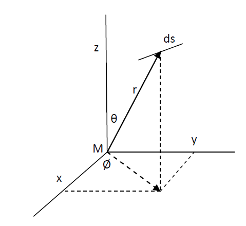
3.3.1 The Chosen Coordinate System and the Local Structure of Space
We work here with a Euclidean coordinate system, which may be interpreted as a Cartesian system (\(t, x, y, z\)) or — as in the Schwarzschild solution — a polar system (\(t, r, θ, ∅\)). In the polar case, the path a particle follows depends on all four coordinates.
The Schwarzschild metric assigns a coefficient to each differential, which is a function of \(r\) and \(θ\), but independent of \(t\) and \(∅\). This reflects the spherical symmetry around the mass \(M\): a rotation about the center changes nothing about the physical situation.
It is important to realize that these coordinates are hypothetical: they are defined as if they existed in a flat, non‑curved spacetime. Schwarzschild found an explicit formula describing the curvature of spacetime around a point mass. This formula relates the infinitesimal line element \(ds\) (the spacetime distance between two neighboring events) to the chosen coordinate system.
Although spacetime is curved, we may treat it locally — in an infinitesimally small region — as flat. Within such a small region, the coordinates \(c dt\), \(dr\), \(dθ\), and \(d∅\) may be treated as mutually orthogonal and linear. The coefficients in the metric can be considered constant there. When we move to another location, these properties remain locally valid, but with different coefficients due to changes in \(r\) and \(θ\).
By then integrating over \(ds\) along a path — that is, summing all infinitesimal steps — we obtain the full trajectory of the particle in curved spacetime.
3.3.2 The Schwarzschild Metric and the Role of Proper Time
As discussed earlier, the Schwarzschild metric in polar coordinates has the form:
\[ ds^2 = c^2 d\tau^2 = \left(1 - \frac{2GM}{c^2 r}\right)c^2 dt^2 - \left(1 - \frac{2GM}{c^2 r}\right)^{-1} dr^2 - r^2 d\theta^2 - r^2 \sin^2\theta\, d\phi^2 \tag{1} \]Here, \( ds^2 \) describes the squared interval in spacetime between two neighboring events.
For compactness, we introduce the function:
\[ \sigma = \sqrt{\,1 - \frac{2GM}{c^2 r}\,} \]which allows the metric to be elegantly rewritten as:
\[ ds^2 = c^2 d\tau^2 = \sigma^2 c^2 dt^2 - \sigma^{-2} dr^2 - r^2 d\theta^2 - r^2 \sin^2\theta\, d\phi^2 \tag{1a} \]Here, \( d\tau \) is the proper time: the time measured by a clock moving with the object. This is the actual duration experienced by an observer along their own worldline.
The coordinate time \( dt \), on the other hand, belongs to a hypothetical system in which no mass is present — an ideal “flat” reference frame. Strictly speaking, \( dt \) is not directly measurable except in the limit \( r \to \infty \), where \( \sigma \to 1 \) and spacetime becomes flat.
Locally, at a fixed value of \( r \), the Schwarzschild metric relates coordinate time and proper time through a simple relation:
\[ \Delta t_{\text{coordinate}} = \sigma\, dt \]where \( \sigma \) depends on the position \( r \).
3.3.3 Distance Traveled, Velocity, and the Relation to the Schwarzschild Metric
In Schwarzschild spacetime, the infinitesimal spatial distance Δdistance between two events is given by:
\[ \Delta \textit{distance} =\sqrt{ \sigma^{-2} dr^2 + r^2 d\theta^2 + r^2 \sin^2\theta\, d\phi^2 } \]Where, as mentioned earlier:
\[ \sigma = \sqrt{\,1 - \tfrac{2GM}{c^2 r}\,} \]The corresponding time duration in coordinate time is:
\[ \Delta \textit{time} = \sigma\, dt \]From this, the (local) velocity \( v \) of a particle in the frame follows:
\[ \frac{v^2}{c^2} = \frac{1}{c^2} \left(\frac{\Delta \textit{distance}}{\Delta \textit{time}} \right)^2 = \frac{\sigma^{-2} dr^2 + r^2 d\theta^2 + r^2 \sin^2\theta\, d\phi^2}{\sigma^2 c^2 dt^2} \]This expression incorporates the curvature of spacetime.
Substituting this expression back into the compact form of the Schwarzschild metric (equation (1a)), we find:
\[ ds^2 = c^2 d\tau^2 = \sigma^2 c^2 dt^2 - \frac{\sigma^{-2} dr^2 + r^2 d\theta^2 + r^2 \sin^2\theta\, d\phi^2}{\sigma^2 c^2 dt^2}\, \sigma^2 c^2 dt^2 \tag{2} \]which simplifies to:
\[ c^2 d\tau^2 = \sigma^2 c^2 dt^2 \left[ 1 - \frac{\sigma^{-4}}{c^2}\left(\frac{dr}{dt}\right)^2 - \frac{\sigma^{-2} r^2}{c^2}\left(\frac{d\theta}{dt}\right)^2 - \frac{\sigma^{-2} r^2 \sin^2\theta}{c^2}\left(\frac{d\phi}{dt}\right)^2 \right] \tag{3} \]or more compactly:
\[ c^2 d\tau^2 = \sigma^2 c^2 dt^2 \left(1 - \frac{v^2}{c^2}\right) \]where:
\[ v^2 = \sigma^{-4}\left(\frac{dr}{dt}\right)^2 + \sigma^{-2} r^2\left(\frac{d\theta}{dt}\right)^2 + \sigma^{-2} r^2 \sin^2\theta\left(\frac{d\phi}{dt}\right)^2 \tag{3a} \]This derivation shows how both spatial and temporal curvature together determine the dynamics of a moving particle.
3.3.4 Relation Between Proper Time and Coordinate Time \( dt \)
From the previous derivation (equation (3)), the relation between proper time \( d\tau \) and coordinate time \( dt \) follows directly:
\[ d\tau = \frac{\sigma}{\gamma} \, dt \]Where:
\[ \sigma = \sqrt{\,1 - \frac{2GM}{c^2 r}\,}, \qquad \gamma = \frac{1}{\sqrt{1 - \frac{v^2}{c^2}}} \tag{4} \]Here, \(\sigma\) measures gravitational time dilation (due to the mass \(M\)), and \(\gamma\) is the Lorentz factor from special relativity.
Because \(\gamma \ge 1\) (since \(v \le c\)) and \(\sigma \le 1\) (since \( r \ge 2GM/c^2 \)), it follows that:
\[ d\tau \le dt \tag{5} \]This means that the proper time of the moving object always runs slower than the coordinate time in the reference frame.
Since both \(\sigma\) and \(\gamma\) are constant during the interval considered (they depend only on \( r \) and \( v \), not on \( t \)), we can integrate this relation easily:
\[ \tau = \frac{\sigma}{\gamma} \, t \tag{5a} \]where \(\tau\) is the elapsed proper time and \( t \) is the elapsed coordinate time.
Thus:
- \(t\) is the coordinate time of an external observer (e.g., someone far from the gravitational field).
- \(\tau\) is the proper time of the particle itself.
And:
- \(\frac{dt}{d\tau}\) = the rate at which coordinate time passes relative to the particle’s proper time.
- \(\frac{dt}{d\tau}\) is not a velocity in meters per second like \(\frac{dr}{dt}\), but a relative “time‑speed” between the observer’s coordinate time and the particle’s proper time.
- It does play the same role in the Lagrangian as a kinetic term: the square \(dt^2\) appears in the energy‑like conserved quantity.
3.3.5 Behavior of a Photon in the Schwarzschild Metric
For a photon, the proper time \( d\tau \) is zero, because a photon always moves at the speed of light:
\[ 0 = \sigma^2 c^2 dt^2 - \sigma^{-2} dr^2 - r^2 d\theta^2 - r^2 \sin^2\theta \, d\phi^2 \tag{6} \]From this, the spatial distance traveled by the photon is:
\[ \left(\Delta \textit{distance}\right)^2 = \sigma^{-2} dr^2 + r^2 d\theta^2 + r^2 \sin^2\theta \, d\phi^2 \tag{6b} \]The effective speed \( v \) of light relative to the chosen coordinate system is then:
\[ c^2 = \left(\frac{\Delta \textit{distance}^2}{\Delta \textit{time}} \right)^2 = \frac{\sigma^{-2} dr^2 + r^2 d\theta^2 + r^2 \sin^2\theta \, d\phi^2}{\sigma^2 dt^2} = v^2 \tag{6c} \]Here, \(\Delta \textit{time} = \sigma dt\), as discussed earlier.
3.3.6 Interpretation
- The numerator contains the “normal” spatial distance the photon travels.
- The denominator shows that *time* is affected by a factor \(\sigma\): the clock at a given location ticks more slowly due to gravity.
This shows that, measured in coordinate time \( dt \), the effective speed of light is lower than \( c \) in the presence of gravity. In the local (co‑moving) frame, of course, the photon still moves at the constant speed \( c \).
3.3.7 Alternative Description of Photon Motion
We can rewrite the relation between distance traveled and elapsed time as:
\[ c^2 =\left(\frac{\Delta \textit{distance}}{\Delta \textit{time}} \right)^2 = \frac{\sigma^{-2}\left(\sigma^{-2} dr^2 + r^2 d\theta^2 + r^2 \sin^2\theta \, d\phi^2\right)}{dt^2} \tag{6d} \]We note:
- The spatial distance is increased by a factor \(\sigma^{-2}\) (since \(\sigma \le 1\)).
- At the same time, the coordinate time \( dt \) remains unchanged.
3.3.8 Consequence
Because the distance in the numerator is increased, while the time in the denominator is unchanged, the speed of light in the coordinate system appears smaller than the universal speed \( c \).
3.3.9 Summary
From the perspective of the “universal” coordinate system:
- A photon moves along a curve in curved spacetime, and
- The effective speed of the photon between two coordinate points (e.g., from A to B) is less than \( c \).
In the expression:
\[ \sigma^2 c^2 = \frac{\sigma^{-2} dr^2 + r^2 d\theta^2 + r^2 \sin^2\theta\, d\phi^2}{dt^2} \tag{6e} \]we see that the speed of light is effectively modified by the factor \(\sigma^2\).
3.3.10 Behavior
This means physically that:
- The intrinsic speed of the photon remains \( c \) along its worldline.
- But the projection of its motion onto the coordinate system appears as a lower speed due to spacetime curvature.
In other words:
\[ v = \frac{\textit{distance}}{\textit{t}} = \frac{\textit{distance}}{\textit{path length}/c} =\frac{\textit{distance}}{\textit{path length}}c \]Because the path length is greater than the “straight distance,” we have \( v < c \) when measured in coordinate time.
3.3.11 Relation Between Local Time on Earth and the Universal Frame Time
As noted earlier, coordinate time \( dt \) is a hypothetical time defined in a massless environment or at infinite distance \( r = \infty \). Since we perform our measurements from Earth, we must relate:
- the proper time \( d\tau_{\textit{earth}} \) measured by a clock on Earth, and
- the coordinate time \( dt \) from the universal reference frame.
As derived earlier (see also equation (5a)), we have:
\[ d\tau_{\text{earth}} = \frac{\sigma_{\textit{earth}}}{\gamma_{\textit{earth}}} \, dt \]Or, equivalently:
\[ dt = \frac{\gamma_{\textit{earth}}}{\sigma_{\textit{earth}}} \, d\tau_{\textit{earth}} \]where:
- \(\sigma_{\textit{earth}} =\sqrt{ 1 - \frac{2GM}{c^2 r_{\textit{earth}}}}\) is the gravitational time‑dilation factor,
- \(\gamma_{\textit{earth}} = \frac{1}{\sqrt{1 - v_{\textit{earth}}^2 / c^2}}\) is the special‑relativistic Lorentz factor (due to Earth’s rotation).
3.3.12 Interpretation
The time on Earth slows down relative to the universal frame due to two effects:
- Gravity (gravitational time dilation, via \(\sigma\)),
- the motion of the Earth (special relativity, via \(\gamma\)).
For an observer moving along with the Earth, their own proper time \( d\tau_{\text{earth}} \) of course proceeds normally — every second is still a second. However, relative to the universal frame time \( dt \), the local seconds run slightly slower.
3.3.13 Summary
- On Earth: the local clock runs normally (i.e., according to \( d\tau \)).
- Relative to the universal frame: the local clock is slowed by gravitational and kinematic effects.
3.3.14 Behavior of a Photon in the Schwarzschild Metric
A special case arises when we consider a photon. Because a photon always travels at the speed of light \( c \) and has no rest mass, the proper time \( d\tau \) along its worldline is equal to zero:
\[ d\tau = 0 \]This also follows directly from the Schwarzschild metric:
\[ 0 = \sigma^2 c^2 dt^2 - \sigma^{-2} dr^2 - r^2 d\theta^2 - r^2 \sin^2\theta\, d\phi^2 \tag{6} \]From this we can deduce that the spatial distance travelled by the photon is:
\[ (\Delta \textit{distance})^2 = \sigma^{-2} dr^2 + r^2 d\theta^2 + r^2 \sin^2\theta\, d\phi^2 \tag{6b} \]and the speed of the photon is:
\[ c^2 = \left(\frac{\Delta \textit{distance}}{\Delta \textit{time}}\right)^2 = \frac{\sigma^{-2} dr^2 + r^2 d\theta^2 + r^2 \sin^2\theta\, d\phi^2}{\sigma^2 dt^2} \tag{6c} \]3.3.15 Remark
Although a photon would have “zero distance” in its own (nonexistent) rest frame, an external observer does see a spatial distance travelled along a curved path in spacetime.
3.3.16 Special Cases
- Radial motion of the photon (only the r-direction, \( d\tau = d\theta = d\phi = 0 \))
Then the previous equation simplifies to:
\[ c^2 = \sigma^{-4} \left(\frac{dr}{dt}\right)^2 \]or
\[ \sigma^4 c^2 dt^2 = dr^2 \]or
\[ \sigma^{-2} \frac{\sigma^{-2} dr}{dt} = c \tag{7} \] - Circular motion in the equatorial plane \(\left( \theta = \pi/2 \right)\)
If the photon moves in a circular orbit around the mass \( M \) (\( d\tau = dr = d\theta = 0 \)), then:
\[ v = c = \frac{r\, d\phi}{\sigma\, dt} \]This shows that the angular velocity \( d\phi/dt \) depends on the distance \( r \) and the curvature factor \(\sigma\).
3.3.17 At Large Distance
If \( r = \infty \), then:
\[ \sigma \to 1 \]and therefore:
\[ d\tau = dt \]The time measured along the photon’s path and the coordinate time coincide — exactly as expected in a region without gravity (flat spacetime).
3.3.18 Summary
- For a photon, \( d\tau = 0 \) always.
- The relation between space and time is fully determined by the curvature factor \(\sigma\).
- In strongly curved spacetime (near mass), the behavior of a photon differs significantly from what we intuitively expect in flat spacetime.
In general, motion at infinite distance is straight and uniform, and the metric becomes:
\[ ds^2 = c^2 d\tau^2 = c^2 dt^2 - dr^2 - r^2 d\theta^2 - r^2 \sin^2\theta\, d\phi^2 \tag{8} \]3.3.19 Transformation to Cartesian Coordinates
Schwarzschild’s original derivation was not in polar coordinates, but in Cartesian coordinates. The transformation yields:
\[ ds^2 = c^2 d\tau^2 = \sigma^2 c^2 dt^2 - dx^2 - dy^2 - dz^2 - \frac{1 - \sigma^2}{\sigma^2 r^2} (x\,dx + y\,dy + z\,dz)^2 \tag{9} \]Where:
- \(\sigma = \sqrt{1 - \frac{2GM}{c^2 r}}\)
- \( r = \sqrt{x^2 + y^2 + z^2} \) is the usual radial distance.
3.3.20 Explanation
The first term \( \sigma^2 c^2 dt^2 \) describes the time component affected by gravity. The second term \( dx^2 + dy^2 + dz^2 \) corresponds to flat spacetime. The third term corrects for the fact that gravitational time dilation also affects spatial components, depending on the direction of motion relative to the mass \( M \).
3.3.21 Note on Differentiating with Respect to t or τ
- Time \( t \) is the coordinate time, measured by an observer at infinite distance (or in a region without mass).
- Time \( \tau \) is the proper time, measured along the worldline of the moving object.
For the plane \( \theta = \pi/2 \) and dividing by \( c^2 d\tau^2 \):
\[ 1 = \sigma^2 \left(\frac{dt}{d\tau}\right)^2 - \sigma^{-2} \left(\frac{dr}{c\, d\tau}\right)^2 - r^2 \left(\frac{d\phi}{c\, d\tau}\right)^2 \tag{10} \]or, rewritten using derivatives with respect to \( t \):
\[ 1 = \sigma^2 \left(\frac{dt}{d\tau}\right)^2 - \sigma^{-2} \left(\frac{dr}{c\, dt} \frac{dt}{d\tau}\right)^2 - r^2 \left(\frac{d\phi}{c\, dt} \frac{dt}{d\tau}\right)^2 \tag{10} \]Then:
\[ 1 = \sigma^2 \left(\frac{dt}{d\tau}\right)^2 \left[ 1 - \frac{1}{\sigma^4} \left(\frac{dr}{c\, dt}\right)^2 - \frac{r^2}{\sigma^2} \left(\frac{d\phi}{c\, dt}\right)^2 \right] \tag{11} \]This shows how motions (velocities) and time dilations in curved spacetime are related.
3.3.22 Speed Relative to Local and Universal Time
The speed relative to the proper time \( \tau \) is:
\[ v_{\text{co}}^2 = \frac{\sigma^{-2} dr^2 + r^2 d\theta^2 + r^2 \sin^2\theta\, d\phi^2}{d\tau^2} \]and the Schwarzschild metric can be written in terms of \( v_{\text{co}} \):
\[ c^2 d\tau^2 = \sigma^2 c^2 dt^2 - v_{\text{co}}^2 d\tau^2 \]Or rewritten:
\[ c^2 d\tau^2 + v_{\text{co}}^2 d\tau^2 = \sigma^2 c^2 dt^2 \]Approximation for small speeds \( (v_{\text{co}} \ll c) \) using a Taylor expansion:
\[ d\tau^2 = \frac{\sigma^2}{1 + (v_{\text{co}}/c)^2} dt^2 \approx \sigma^2 \left(1 - \frac{v_{\text{co}}^2}{c^2}\right) dt^2 \] \[ d\tau \approx \sigma \sqrt{1 - \frac{v_{\text{co}}^2}{c^2}}\, dt \quad\Rightarrow\quad d\tau = \frac{\sigma}{\gamma_{\text{co}}} dt \]with \( \gamma_{\text{co}} = \dfrac{1}{\sqrt{1 - v_{\text{co}}^2/c^2}} \).
3.3.23 Summary
- Schwarzschild originally worked in Cartesian coordinates.
- The Schwarzschild metric can be expressed in both spherical and Cartesian form.
- When interpreting motion, it is essential to distinguish between coordinate time \( t \) and proper time \( \tau \).
- For small speeds, the influence of spacetime curvature on time is small but measurable.
In general, a trajectory lies in a single plane. The polar system can then be chosen such that the equatorial plane coincides with the trajectory plane (\( \theta = \pi/2 \)). If the trajectory is circular (\( r \) constant), then \( dr = 0 \) and:
\[ c^2 d\tau^2 = \sigma^2 c^2 dt^2 - r^2 d\phi^2 \]Below follow additional considerations:
3.3.24 Supplement 1: Interpretation of ds as a Line Segment in Spacetime
It may be useful to think of ds as an infinitesimal line segment in spacetime, whose length in meters can be measured by multiplying the travel time of a photon across that segment by the speed of light c. The line segment ds is located at the origin of its own comoving reference frame. Within that frame, time is the only physical quantity that can be directly measured. Distance is measured via the photon’s travel time.
Thus:
\[ ds = c\, d\tau \]where \( d\tau \) is the proper time recorded by a comoving clock.
Now we introduce a second reference frame, for example the Schwarzschild frame, in which a central mass M is present. In this frame we can determine the distance between the line segment and the origin using external measuring devices (lasers, rods, etc.).
Important:
The time measurement in this external frame is indirect: it depends on the relation given
by the Schwarzschild metric, and cannot be measured directly by a local clock.
According to the Schwarzschild metric:
\( c^{2} d\tau^{2} = (c \Delta T)^{2} - (\Delta X)^{2} \)
\( (c \Delta T)^{2} = \left(1 - \dfrac{2GM}{c^{2} r}\right) c^{2} dt^{2} = c^{2} d\tau^{2} - (\Delta X)^{2} \)
where the spatial component is:
\( (\Delta X)^{2} = \dfrac{1}{1 - \dfrac{2GM}{c^{2} r}}\, dr^{2} + r^{2} d\theta^{2} + r^{2} \sin^{2}\theta\, d\phi^{2} \)
From this follows:
\( c^{2} dt^{2} = \dfrac{(c \Delta T)^{2}}{1 - \dfrac{2GM}{c^{2} r}} \)
The relation between the theoretical time dt and the proper time \( d\tau \) can only be determined through this formula.
3.3.25 Supplement 2: Worldline of a Particle in a Comoving Reference Frame
When we consider a particle in a comoving (local) reference frame, the particle is at rest with respect to that frame. The only path the particle follows in spacetime is along its own τ-axis: the proper time.
However, we can describe the motion of the particle with respect to an external (possibly moving) reference frame. In that case, we express the position of the particle in the coordinates \((t, x, y, z)\) of that other frame.
The worldline of the particle — the path it follows through spacetime — is then entirely a function of \(\tau\):
\[ t(\tau), x(\tau), y(\tau), z(\tau) \]The four coordinates are therefore functions of the proper time \(\tau\).
3.3.26 Example: Time Difference Between the Poles and the Equator
We compute the time difference at Earth’s surface between the time at the poles and at the equator, caused by relativistic effects.
Starting from the Schwarzschild metric:
\[ c^2 d\tau^2 = \sigma^2 c^2 dt^2 - \sigma^{-2} dr^2 - r^2 d\theta^2 - r^2 \sin^2\theta\, d\phi^2 \]3.3.27 At the Poles
At the poles:
- \(dr = 0\) (no radial motion),
- \(\theta = 0\),
- \(d\theta = 0\),
- \(\sin\theta = 0\).
from which follows:
\[ d\tau_{\textit{poles}} = \sigma dt \]3.3.28 At the Equator
At the equator:
- \(dr = 0\),
- \(\theta = \pi/2\),
- \(d\theta = 0\),
- \(\sin\theta = 1\)
where \(d\phi\) describes the rotation around Earth’s rotation axis.
We rewrite this as:
\[ c^2 d\tau^2_{\textit{equator}} = c^2 d\tau^2_{\textit{poles}} - r^2 d\phi^2 \]Or:
\[ c^2 d\tau^2_{\textit{equator}} = c^2 d\tau^2_{\textit{poles}} \left\{1 - \frac{r^2}{c^2} \left(\frac{d\phi}{d\tau_{\textit{poles}}}\right)^2\right\} \]The rotational speed at the equator is:
\[ v_{\textit{equator}} = r \frac{d\phi}{d\tau_{\textit{poles}}} \]Thus:
\[ c^2 d\tau^2_{\textit{equator}} = c^2 d\tau^2_{\textit{poles}} \left(1 - \frac{v^2_{\textit{equator}}}{c^2}\right) \] and \[ d\tau_{\textit{equator}} = d\tau_{\textit{poles}} \sqrt{1 - \frac{v^2_{\textit{equator}}}{c^2}} \]For small velocities \(v \ll c\), we approximate using a Taylor expansion:
\[ d\tau_{\textit{equator}} \approx d\tau_{\textit{poles}} \left(1 - \frac{1}{2}\frac{v^2_{\textit{equator}}}{c^2}\right) \]3.3.29 Practical Calculation
The rotational speed at the equator is approximately:
\[
\approx 1672\ \text{km/h} \quad \text{or} \quad 465\ \text{m/s}
\]
This yields:
\[
\frac{v^2_{\textit{equator}}}{c^2} \approx 2.4 \cdot 10^{-12}
\]
Thus:
\[
d\tau_{\textit{equator}} = d\tau_{\textit{poles}} \sqrt{1 - 2.4 \cdot 10^{-12}}
\]
3.3.30 Interpretation
A clock at the equator ticks slightly slower than a clock at the poles. Over a period of 100 years, the difference accumulates to approximately:
100 years × 1.2·10⁻¹² ≈ 3.75 milliseconds
3.3.31 Conclusion
A person who lived 100 years at the North Pole would (theoretically) be about 3.75 milliseconds older than someone who lived at the equator, assuming all other conditions remained equal.
3.3.32 Supplement 3: The Schwarzschild Coefficient and the Escape Velocity
Let us pay special attention to the factor:
\[ 1 - \frac{2GM}{c^2 r} \]This expression resembles the well‑known formula for the escape velocity, which determines the minimum speed a mass must have to escape another mass (e.g., Earth).
3.3.33 Calculation of the Minimum Escape Velocity
Consider a mass m being launched away from an object of mass M (e.g., Earth). Then:
- The kinetic energy of m: \[ E_{\text{kin}} = \frac{1}{2} m v^2 \]
- The gravitational force on m: \[ F = \frac{G M m}{r^2} \] where r is the distance to the center of mass M.
- The work required to move m from r to infinity (where gravity vanishes) is: \[ W = \int_r^\infty F\, ds = \int_r^\infty \frac{G M m}{s^2}\, ds \] \[ = G M m \left(\frac{1}{r} - \frac{1}{\infty}\right) = \frac{G M m}{r} \]
To escape, the kinetic energy must equal this work:
\[ \frac{1}{2} m v^2 = \frac{G M m}{r} \]Thus:
\[ v^2 = \frac{2 G M}{r} \] \[ v = \sqrt{\frac{2 G M}{r}} \]Or inversely:
\[ r = \frac{2 G M}{v^2} \]3.3.34 The Maximum Speed: Light
The maximum possible speed is the speed of light c. If v = c, then:
\[ r = \frac{2 G M}{c^2} \]This is the Schwarzschild radius:
\[ r = R_s = \frac{2 G M}{c^2} \]When an object lies within this radius, escape is impossible — even light cannot escape. In that case, we speak of a black hole.
3.3.35 Relation to the Schwarzschild Metric
In the Schwarzschild metric, this radius appears in the factor:
\[ 1 - \frac{2 G M}{c^2 r} \]Normally this factor lies between 1 and 0:
- At large distances \(r \to \infty\), the factor approaches 1.
- At the Schwarzschild radius \(r = R_s\), the factor becomes 0.
When \(1 - 2GM/(c^2 r) = 0\), the object is exactly at the Schwarzschild radius — the event horizon of a black hole.
3.3.36 Remark
If \(r\) becomes smaller than \(R_s\), the factor becomes negative. The physical meaning of this requires deeper analysis within the relativistic theory of black holes and lies beyond the scope of this section.
3.3.37 Key Points and Intuition
- In general relativity, geometry replaces force: mass curves spacetime instead of generating a force field.
- The Schwarzschild metric describes this curvature around a spherically symmetric mass and applies outside the mass, where \(T_{\mu\nu} = 0\).
- A test particle moving in this field feels no force but follows a geodesic — the “straightest” path in curved spacetime.
- The metric in spherical coordinates: \[ ds^2 = c^2 d\tau^2 = \sigma^2 c^2 dt^2 - \sigma^{-2} dr^2 - r^2 d\theta^2 - r^2 \sin^2\theta\, d\phi^2 \] with \[ \sigma = \sqrt{1 - \frac{2GM}{c^2 r}} \]
- The coordinate time \(dt\) applies in the asymptotically flat (hypothetical) frame at \(r \to \infty\); the proper time \(d\tau\) is measured by a clock comoving with the object.
Intuitively: Einstein states that a mass affects the measurement structure of space and time itself. A freely falling object does not move “because of a force,” but follows the path imposed by the geometry of spacetime — like a pebble rolling along a curved surface.
- Time runs slower closer to a mass (via \(σ < 1\)).
- Space is stretched in the radial direction.
- For a moving object, the metric relates \(d\tau\) to \(dt\) and its speed \(v\):
\(d\tau =\frac{ \sigma}{\gamma} dt,\) with \(\gamma = 1 / \sqrt{1 - v^2/c^2}\)
Table: Concepts and Physical Quantities from the Schwarzschild Metric
| Quantity | Physical Interpretation |
|---|---|
| \(\sigma=\sqrt{ 1 - 2GM/(c² r)}\) | Gravitational time dilation factor |
| dτ | Proper time: measured by a local clock |
| dt | Coordinate time: measured in an asymptotically flat frame |
| v | Local speed, derived from spatial coordinates and dt |
| ds² = c² dτ² | Four‑dimensional interval (invariant): time and space element |
| R_s = 2GM/c² | Schwarzschild radius: where σ = 0, event horizon |
3.3.38 Specific Cases and Effects
- Photons:
- Follow a trajectory with \(d\tau = 0\): they experience no proper time.
- The effective speed of light in coordinate time is less than \(c\) (but locally \(v = c\)).
- Object at rest near a mass:
- Time dilation via \(d\tau = \frac{\sigma}{\gamma} dt\): the smaller \(r\), the slower the clock.
- Object in motion (e.g., circular orbit):
- Both gravitational and kinematic time dilation play a role.
- Velocity in Schwarzschild coordinates:
\[ v^2 = \sigma^{-4} \left(\frac{dr}{dt}\right)^2 + \sigma^{-2} r^2 \left(\frac{d\theta}{dt}\right)^2 + \sigma^{-2} r^2 \sin^2\theta \left(\frac{d\phi}{dt}\right)^2 \tag{3a} \]
3.3.39 Application: Time on Earth vs. Time at Infinity
- Time on Earth runs slower relative to the universal coordinate time, due to:
- gravity (via \(σ\)),
- Earth’s rotation (via \(γ\)).
- Result: over 100 years, a clock at the poles is ≈ 3.75 ms ahead of a clock at the equator (approximate).
3.3.40 Black Holes and Escape Velocity
- From Newtonian mechanics:
\(v_{\text{escape}} = \sqrt{\frac{2 G M}{r}} \;\Rightarrow\; R_s = \frac{2 G M}{c^2}\)
- At \(r = R_s\), \(σ \to 0\) (event horizon): nothing can escape.
- The Schwarzschild metric contains this boundary explicitly.
3.3.41 Slotinzicht
De Schwarzschild-metriek levert direct meetbare voorspellingen:
- Tijdsdilatatie (o.a. GPS-correcties)
- Lichtafbuiging (zoals gemeten tijdens zonsverduisteringen)
- Periheliumprecessie van Mercurius
- Voorwaarden voor het ontstaan van zwarte gaten
De Schwarzschild-metriek is dus geen abstract wiskundig object, maar een fysische machine die ons vertelt hoe klokken lopen, hoe licht buigt, en hoe massa’s bewegen - puur op basis van de geometrie van ruimte en tijd.
3.4 Experimenten: Bevestiging van de Algemene Relativiteit
De algemene relativiteitstheorie is niet alleen een elegante wiskundige theorie, maar wordt ook krachtig ondersteund door experimenten en waarnemingen. Veel van deze experimenten maken gebruik van de Schwarzschild-oplossing als basis voor hun theoretische voorspellingen. De volgende experimenten worden in dit werk besproken:
- Hafele-Keating-experiment (1971) (zie hoofdstuk 4.1)
- Beschrijving: Atoomklokken werden in vliegtuigen rond de aarde gevlogen, zowel oostwaarts als westwaarts, en vergeleken met klokken op de grond.
- Resultaat: De gemeten tijdsverschillen kwamen exact overeen met de voorspellingen van de algemene relativiteit (zwaartekrachts-tijdsdilatatie én bewegings-tijdsdilatatie).
- Relatie tot Schwarzschild-metriek: De tijdsdilatatie door zwaartekracht wordt direct uit de Schwarzschild-oplossing afgeleid.
- Beweging van deeltjes in een zwaartekrachtveld (zie hoofdstuk 4.2)
- Beschrijving: De banen van satellieten, planeten en andere objecten worden nauwkeurig gevolgd.
- Resultaat: De waargenomen banen komen overeen met de voorspellingen uit de Schwarzschild-geometrie, inclusief kleine afwijkingen van de klassieke (Newtonse) voorspellingen.
- Afbuiging van licht nabij massa’s (zie hoofdstuk 4.3)
- Beschrijving: Tijdens zonsverduisteringen werd gemeten hoe het licht van sterren wordt afgebogen door de zwaartekracht van de zon.
- Resultaat: De gemeten afbuiging (door Eddington in 1919 en vele latere experimenten) komt exact overeen met de waarde voorspeld door de Schwarzschild-metriek.
- Fysisch belang: Bewijst dat licht zelf wordt beïnvloed door de kromming van ruimte-tijd.
- Precessie van de periheliën (Mercurius) (zie hoofdstuk 4.4)
- Beschrijving: De baan van Mercurius draait langzaam rond de zon; deze precessie kan niet volledig door Newtonse zwaartekracht verklaard worden.
- Resultaat: De resterende precessie wordt exact verklaard door de Schwarzschild-oplossing.
- Historisch belang: Dit was een van de eerste grote successen van de algemene relativiteit.
- Shapiro-tijdvertraging (zie hoofdstuk 4.5)
- Beschrijving
3.3.41 Final Insight
The Schwarzschild metric provides directly measurable predictions:
- Time dilation (e.g., GPS corrections)
- Light deflection (as measured during solar eclipses)
- Perihelion precession of Mercury
- Conditions for the formation of black holes
The Schwarzschild metric is therefore not an abstract mathematical object, but a physical machine that tells us how clocks run, how light bends, and how masses move — purely based on the geometry of space and time.
3.4 Experiments: Confirmation of General Relativity
The general theory of relativity is not only an elegant mathematical theory, but is also strongly supported by experiments and observations. Many of these experiments use the Schwarzschild solution as the basis for their theoretical predictions. The following experiments are discussed in this work:
- Hafele–Keating experiment (1971) (see Chapter 4.1)
- Description: Atomic clocks were flown around the Earth in airplanes, both eastward and westward, and compared with clocks on the ground.
- Result: The measured time differences matched exactly the predictions of general relativity (gravitational time dilation and kinematic time dilation).
- Relation to Schwarzschild metric: The gravitational time dilation is derived directly from the Schwarzschild solution.
- Motion of particles in a gravitational field (see Chapter 4.2)
- Description: The orbits of satellites, planets, and other objects are tracked with high precision.
- Result: The observed orbits match the predictions from Schwarzschild geometry, including small deviations from classical (Newtonian) predictions.
- Deflection of light near massive bodies (see Chapter 4.3)
- Description: During solar eclipses, the bending of starlight by the Sun’s gravity was measured.
- Result: The measured deflection (by Eddington in 1919 and many later experiments) matches exactly the value predicted by the Schwarzschild metric.
- Physical significance: Demonstrates that light itself is influenced by the curvature of space-time.
- Perihelion precession of Mercury (see Chapter 4.4)
- Description: Mercury’s orbit slowly rotates around the Sun; this precession cannot be fully explained by Newtonian gravity.
- Result: The remaining precession is explained exactly by the Schwarzschild solution.
- Historical significance: One of the first major successes of general relativity.
- Shapiro time delay (see Chapter 4.5)
- Description: Radio waves traveling near the Sun take longer than expected in flat space-time.
- Result: The extra delay matches the prediction of the Schwarzschild metric.
- Application: Used in radar and communication satellites.
- Trajectory of a projectile in a strong gravitational field (see Chapter 4.8)
- Description: Simulations and measurements of objects moving at high speed near massive bodies.
- Result: The trajectories deviate from Newtonian predictions but match the Schwarzschild predictions.
Conclusion
In all these experiments, the results are in excellent agreement with the predictions of general relativity, as derived from the Schwarzschild metric. This forms a powerful confirmation of the correctness of Einstein’s theory.
Key Point
General relativity is not only a mathematically elegant theory, but is also experimentally confirmed to high precision. The Schwarzschild metric is the key to understanding most classical tests of gravity.
- Beschrijving