Chapter 5 – Coordinate Systems | Einstein’s General Theory of Relativity

Part V – Coordinates and Formal Analysis

5 Coordinate Systems

5.1 Rectangular (Cartesian) Coordinate System

To distinguish between points in space, a coordinate system is created. The main characteristics of a coordinate system are the origin and the coordinate axes. The origin can be chosen based on what is most practical, and for the axes, a Cartesian system is usually chosen because of its simplicity and mathematical convenience.

In a Cartesian coordinate system:

The axes are perpendicular (orthogonal) to each other.
The axes are independent of each other, i.e., changing the value of one coordinate does not affect the others.
The axes have direction and magnitude and can therefore be considered as vectors.

A point in space is represented by its coordinates, for example \( A(x_a, y_a) \). The \( x_a \) can be found by drawing a line parallel to the y-axis; where that line intersects the x-axis lies the point \( x_a \). The same applies to \( y_a \).

The distance from point A to the origin can be found using Pythagoras:

\begin{equation} |A - O_{\text{oorsprong}}|^{2} = x_a^{2} + y_a^{2}. \end{equation}

If we work with a line segment between A and B, then the length is:

\begin{equation} |A - B|^{2} = (x_a - x_b)^{2} + (y_a - y_b)^{2}. \end{equation}

The advantage is that the length of the line segment is independent of the chosen origin; i.e., the values of \( x_a, y_a, x_b, y_b \) may change, but the difference \( |A - B| \), which is the length of the segment, does not.

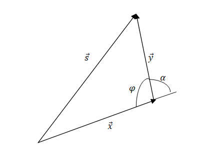
5.2 Non-Orthogonal Coordinate System

For practical reasons, a coordinate system can also be chosen in which the axes are not orthogonal. Positions and distances can still be described in such a system, but the calculations become somewhat more complex.

A line segment \( s \) in this system is the sum of the basis vectors:

\begin{equation} \vec{s} = \,\vec{x} + \,\vec{y}. \end{equation}

The magnitude \( s \) of \( \vec{s} \) can be found by taking the inner product of \( \vec{s} \) with itself:

\begin{equation} \vec{s}\cdot\vec{s} = (\vec{x} + \vec{y}) \cdot (\vec{x} + \vec{y}) = (\vec{x}\cdot\vec{x}) + (\vec{x}\cdot\vec{y}) + (\vec{y}\cdot\vec{x}) + (\vec{y}\cdot\vec{y}) \end{equation}

\begin{equation} =x^2+2(\vec{x}\cdot\vec{y})+y^2 \end{equation}

Thus:

\begin{equation} s^{2} = x^{2} + 2xy\cos\alpha + y^{2}. \end{equation}

If \( \varphi \) is the angle between \( x \) and \( y \), then:

\begin{equation} \cos\alpha = -\cos\varphi, \qquad \cos\alpha = \cos(180^\circ - \varphi) = -\cos\varphi. \end{equation}

Thus:

\begin{equation} s^{2} = x^{2} + y^{2} - 2xy\cos\varphi. \end{equation}

This is the well-known cosine rule. Thus, in addition to the squares of the coordinates, the product of the coordinates also appears in the equation.

5.3 Curved Coordinates

Instead of coordinate axes that are not orthogonal, it may also be practical to use curved coordinates. Working with these coordinates is naturally more complex, but Einstein used the following approach:

A curved line can be considered as a line composed of infinitely small straight segments. By looking at an infinitesimally small region, these curved coordinates can be treated as a local coordinate system with straight (linear) coordinates, which are not necessarily rectangular.

Because the coordinate system here involves infinitesimal coordinates, they are denoted as \( dx, dy \), etc. Moreover, these coordinates have coefficients, and these coefficients contain information about the curvature of the coordinate systems. In the case of curvature, these coefficients are therefore no longer constants, but parameters that depend on their position along the coordinate systems.

It is said that gravity bends coordinate systems and thereby deforms spacetime, creating a gravitational field and thus causing acceleration. However, by choosing a curved coordinate system that moves and bends along with the gravitational field, no force or gravity is experienced; in the same way as in special relativity a moving coordinate system was chosen to neutralize the velocity of the moving object.

5.4 General Form for a Coordinate System

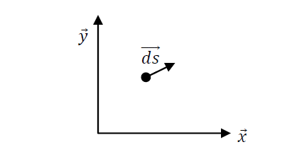
Let us derive an expression for the relation between a line segment and its curved coordinate system.

As mentioned earlier, an infinitesimal line segment \( d\vec{s} \) is a vector, and its magnitude can be calculated as shown above:

\begin{equation} d\vec{s}\cdot d\vec{s} = (d\vec{x} + d\vec{y})\cdot(d\vec{x} + d\vec{y}) = d\vec{x}\cdot d\vec{x} + d\vec{x}\cdot d\vec{y} + d\vec{y}\cdot d\vec{x} + d\vec{y}\cdot d\vec{y}, \end{equation}

for a linear, non-orthogonal system.

To obtain a more general form (not necessarily orthogonal), it is assumed that each term has a coefficient \( g_{\mu\nu} \):

\begin{equation} ds^{2} = g_{xx}\,dx\,dx + g_{xy}\,dx\,dy + g_{yx}\,dy\,dx + g_{yy}\,dy\,dy. \end{equation}

Here, in the example of the cosine rule above:

\begin{equation} g_{xx} = g_{yy} = 1, \qquad g_{xy} = g_{yx} = -\cos\varphi. \end{equation}

The \( g_{\mu\nu} \) is called the metric tensor and, in this two-dimensional coordinate system, can be considered as a matrix with 2×2 elements:

\begin{equation} g_{\mu\nu} = \begin{pmatrix} 1 & -\cos\varphi \\ -\cos\varphi & 1 \end{pmatrix}. \end{equation}

5.5 The Metric Tensor and Einstein Notation

For a general four-dimensional spacetime system (with time as coordinate \( ct \)), the metric is a 4×4 tensor. The general form is:

\begin{equation} ds^{2} = \sum_{\mu=0}^{3}\sum_{\nu=0}^{3} g_{\mu\nu}\,dx^{\mu}\,dx^{\nu} \end{equation}

In Einstein notation:

\begin{equation} ds^{2} = g_{\mu\nu}\,dx^{\mu}\,dx^{\nu}. \end{equation}

Here \( \mu \) and \( \nu \) run from 0 to 3, with coordinates:

\begin{equation} x^{0} = ct,\qquad x^{1} = x,\qquad x^{2} = y,\qquad x^{3} = z. \end{equation}

The metric tensor \( g_{\mu\nu} \) contains all information about the curvature of spacetime.

Example of a metric tensor in matrix form:

\begin{equation} g_{\mu\nu} = \begin{pmatrix} g_{00} & g_{01} & g_{02} & g_{03} \\ g_{10} & g_{11} & g_{12} & g_{13} \\ g_{20} & g_{21} & g_{22} & g_{23} \\ g_{30} & g_{31} & g_{32} & g_{33} \end{pmatrix}. \end{equation}

If the coordinate system is orthogonal, then all cross terms (where \( \mu \neq \nu \)) are zero:

\begin{equation} g_{\mu\nu} = 0 \quad \text{for } \mu \neq \nu. \end{equation}

The value of \( ds^{2} \) remains unchanged under a change of coordinate system, provided the corresponding metric is correctly adjusted. That is:

\begin{equation} ds^{2} = g_{\mu\nu}(x)\,dx^{\mu}\,dx^{\nu} = g_{\alpha\beta}(y)\,dy^{\alpha}\,dy^{\beta}. \end{equation}

Here you can see that \( g_{\mu\nu} \) acts as the “weighting factor” that determines how the infinitesimal displacements in the \( \mu \)- and \( \nu \)-directions contribute to the length.

The diagonal elements \( g_{\mu\mu} \) can be viewed as the “scale factors” for the corresponding coordinate direction.
The off-diagonal elements \( g_{\mu\nu} \) with \( \mu \neq \nu \) describe whether the coordinate directions are skew (i.e., not perpendicular). In a sense, they are related to direction cosines (projections of one axis onto another).

Summary

A coordinate system is a tool to structure space; distances can be calculated within it.
In orthogonal systems, Pythagoras applies; in non-orthogonal systems, the cosine rule applies.
Curved coordinate systems are required to describe gravitational fields in general relativity.
The metric \( g_{\mu\nu} \) contains all information about distance measurement and curvature of space or spacetime.

5.6 Transformation between Two Coordinate Systems

As mentioned earlier, in a curved coordinate system one can locally, within an infinitesimally small region, use a coordinate system with straight lines. For a four-dimensional coordinate system, each new coordinate in the new \( x \)-system has a linear relation with all old coordinates in the old \( y \)-system, according to:

\begin{equation} dx^{0} = \frac{\partial x^{0}}{\partial y^{0}}\,dy^{0} + \frac{\partial x^{0}}{\partial y^{1}}\,dy^{1} + \frac{\partial x^{0}}{\partial y^{2}}\,dy^{2} + \frac{\partial x^{0}}{\partial y^{3}}\,dy^{3}. \end{equation}

The same applies to the other three coordinates, leading to the general formula:

\begin{equation} dx^{m} = \frac{\partial x^{m}}{\partial y^{r}}\,dy^{r}. \end{equation}

The summation is performed over the repeated index \( r \). This implies summation over the index \( r \) according to Einstein notation. This means that for each value of \( m \), the derivatives over all values of \( r \) (from 0 to 3) are added. This formula describes how an infinitesimal change in the new coordinate system \( x^{m} \) is constructed from changes in the old system \( y^{r} \).

5.6.1 Extended Explanation of the Metric Tensor

We begin with a Cartesian coordinate system, which in this case is comparable to the Minkowski equation (see chapter 5.10.1 and Appendix 9.1 equation (35)) in special relativity:

\begin{equation} ds^{2} = c^{2}dt^{2} - dx^{2} - dy^{2} - dz^{2}. \end{equation}

To make the notation more compact and general, we rename the differential terms:

\begin{equation} cdt = dx^{0},\qquad dx = dx^{1},\qquad dy = dx^{2},\qquad dz = dx^{3}. \end{equation}

Here all differential terms have the dimension of length (meters).

In this notation, the spacetime interval is written as:

\begin{equation} ds^{2} = (dx^{0})^{2} - (dx^{1})^{2} - (dx^{2})^{2} - (dx^{3})^{2} = \eta_{\mu\nu}\,dx^{\mu}\,dx^{\nu}. \end{equation}

The metric tensor \( \eta_{\mu\nu} \) (the Minkowski metric) in matrix form is:

\begin{equation} \eta_{\mu\nu} = \begin{pmatrix} 1 & 0 & 0 & 0 \\ 0 & -1 & 0 & 0 \\ 0 & 0 & -1 & 0 \\ 0 & 0 & 0 & -1 \end{pmatrix}. \end{equation}

This tensor describes the distance structure of flat spacetime. The distance between two events is therefore:

\begin{equation} ds^{2} = \eta_{\mu\nu}\,dx^{\mu}\,dx^{\nu}. \end{equation}

Now we consider an arbitrary coordinate system \( y^{\alpha} \), with coordinates \( y^{0}, y^{1}, y^{2}, y^{3} \). The relation between the old and the new system is given by the chain rule:

\begin{equation} dx^{\mu} = \frac{\partial x^{\mu}}{\partial y^{0}}\,dy^{0} + \frac{\partial x^{\mu}}{\partial y^{1}}\,dy^{1} + \frac{\partial x^{\mu}}{\partial y^{2}}\,dy^{2} + \frac{\partial x^{\mu}}{\partial y^{3}}\,dy^{3}. \end{equation}

Or in compact notation:

\begin{equation} dx^{\mu} = \frac{\partial x^{\mu}}{\partial y^{\alpha}}\,dy^{\alpha}, \qquad dx^{\nu} = \frac{\partial x^{\nu}}{\partial y^{\beta}}\,dy^{\beta}. \end{equation}

Substitution into the Minkowski form:

\begin{equation} ds^{2} = \eta_{\mu\nu}\,dx^{\mu}\,dx^{\nu} \end{equation}

gives:

\begin{equation} ds^{2} = \eta_{\mu\nu} \frac{\partial x^{\mu}}{\partial y^{\alpha}} \frac{\partial x^{\nu}}{\partial y^{\beta}} \,dy^{\alpha}\,dy^{\beta}. \end{equation}

We now define a new metric tensor \( g_{\alpha\beta} \) in the coordinate system \( y^{\alpha} \), as follows:

\begin{equation} g_{\alpha\beta} = \eta_{\mu\nu} \frac{\partial x^{\mu}}{\partial y^{\alpha}} \frac{\partial x^{\nu}}{\partial y^{\beta}}. \end{equation}

So that:

\begin{equation} ds^{2} = g_{\alpha\beta}\,dy^{\alpha}\,dy^{\beta}. \end{equation}

If we then transform to another arbitrary coordinate system \( x^{\mu} \), the inverse transformation holds:

\begin{equation} ds^{2} = g_{\alpha\beta} \frac{\partial y^{\alpha}}{\partial x^{\mu}} \frac{\partial y^{\beta}}{\partial x^{\nu}} \,dx^{\mu}\,dx^{\nu} = g_{\mu\nu}\,dx^{\mu}\,dx^{\nu}. \end{equation}

From this follows the general transformation formula for the metric tensor:

\begin{equation} g_{\mu\nu}(x) = \frac{\partial y^{\alpha}}{\partial x^{\mu}} \frac{\partial y^{\beta}}{\partial x^{\nu}} g_{\alpha\beta}(y). \end{equation}

This formula describes how the components of the metric tensor transform under a general coordinate transformation. It is a fundamental result in general relativity and forms the basis for understanding curved spacetime.

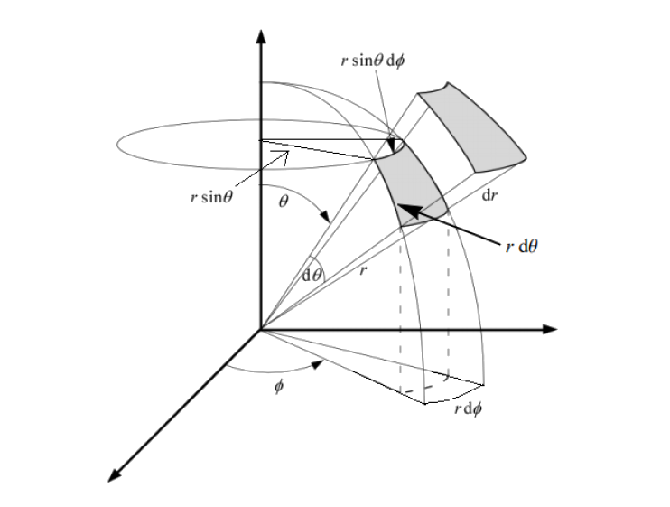
5.7 Transformation between Cartesian and Polar (Infinitesimal) Coordinates

As an example, we now perform the transformation from a Cartesian to a spherical (polar) coordinate system. We assume that the reader is familiar with the standard transformation between the two systems:

\begin{equation} x = r\sin\theta\cos\varphi,\qquad y = r\sin\theta\sin\varphi,\qquad z = r\cos\theta. \end{equation}

Derivation of \( dx, dy, dz \)

We differentiate the above expressions to obtain the infinitesimal displacements:

\begin{equation} d\vec{x} = \begin{cases} \vec{x} = \sin\theta\cos\varphi\,d\vec{r} + r\cos\theta\cos\varphi\,d\vec{\theta} - r\sin\theta\sin\varphi\,d\vec{\varphi}, \\ \vec{y} = \sin\theta\sin\varphi\,d\vec{r} + r\cos\theta\sin\varphi\,d\vec{\theta} + r\sin\theta\cos\varphi\,d\vec{\varphi}, \\ \vec{z} = \cos\theta\,d\vec{r} - r\sin\theta\,d\vec{\theta}. \end{cases} \end{equation}

These vectorial differentials describe the infinitesimal displacements in the x-, y-, and z-directions in terms of \( dr, d\theta, d\varphi \).

Determination of the squares of the differentials

To determine the magnitudes of \(dx\), \(dy\), and \(dz\), we take the inner product of each:

\begin{equation} dx^{2} = d\vec{x} \cdot d\vec{x},\qquad dy^{2} = d\vec{y} \cdot d\vec{y},\qquad dz^{2} = d\vec{z} \cdot d\vec{z}. \end{equation}

Because the coordinates \( r, \theta, \varphi \) are mutually orthogonal, the cross terms vanish, resulting in:

\begin{equation} dx^{2} = \sin^{2}\theta\cos^{2}\varphi\,dr^{2} + r^{2}\cos^{2}\theta\cos^{2}\varphi\,d\theta^{2} + r^{2}\sin^{2}\theta\sin^{2}\varphi\,d\varphi^{2}, \end{equation}

\begin{equation} dy^{2} = \sin^{2}\theta\sin^{2}\varphi\,dr^{2} + r^{2}\cos^{2}\theta\sin^{2}\varphi\,d\theta^{2} + r^{2}\sin^{2}\theta\cos^{2}\varphi\,d\varphi^{2}, \end{equation}

\begin{equation} dz^{2} = \cos^{2}\theta\,dr^{2} + r^{2}\sin^{2}\theta\,d\theta^{2}. \end{equation}

Addition of \(dx^{2} + dy^{2} + dz^{2}\)

By adding the three expressions above, we obtain:

\begin{equation} dx^{2} + dy^{2} + dz^{2} = \sin^{2}\theta\cos^{2}\varphi\,dr^{2} + \sin^{2}\theta\sin^{2}\varphi\,dr^{2} + \cos^{2}\theta\,dr^{2} \end{equation}

\begin{equation} \quad + r^{2}\cos^{2}\theta\cos^{2}\varphi\,d\theta^{2} + r^{2}\cos^{2}\theta\sin^{2}\varphi\,d\theta^{2} + r^{2}\sin^{2}\theta\,d\theta^{2} \end{equation}

\begin{equation} \quad + r^{2}\sin^{2}\theta\sin^{2}\varphi\,d\varphi^{2} + r^{2}\sin^{2}\theta\cos^{2}\varphi\,d\varphi^{2}. \end{equation}

Using the trigonometric identities:

\begin{equation} \cos^{2}\varphi + \sin^{2}\varphi = 1, \qquad \cos^{2}\theta + \sin^{2}\theta = 1, \end{equation}

this simplifies to:

\begin{equation} dx^{2} + dy^{2} + dz^{2} = dr^{2} + r^{2}d\theta^{2} + r^{2}\sin^{2}\theta\,d\varphi^{2}. \end{equation}

This expression is precisely the spatial component of the metric in spherical coordinates. The time component can be added as:

\begin{equation} ds^{2} = c^{2}dt^{2} - dx^{2} - dy^{2} - dz^{2} \end{equation}

or in spherical form:

\begin{equation} ds^{2} = c^{2}dt^{2} - dr^{2} - r^{2}d\theta^{2} - r^{2}\sin^{2}\theta\,d\varphi^{2} \end{equation}

Volume Element in Spherical Coordinates

This describes the transformation from a system with Cartesian coordinates to a system with spherical (polar) coordinates.

Volume Element in Cartesian and Spherical Coordinates

The volume element in Cartesian coordinates is:

\begin{equation} dV = dx\,dy\,dz. \end{equation}

After transformation to spherical coordinates, this becomes:

\begin{equation} dV = dr \cdot (r\,d\theta) \cdot (r\sin\theta\,d\varphi) = r^{2}\sin\theta\,dr\,d\theta\,d\varphi. \end{equation}

Calculation of the Volume of a Sphere

The total volume of a sphere with radius \( R \) follows from the integral:

\begin{equation} V =\iiint r^{2}\sin\theta\,dr\,d\theta\,d\varphi, \end{equation}

with the integration limits:

\( r \in [0, R] \)
\( \theta \in [0, \pi] \)
\( \varphi \in [0, 2\pi] \)

The integral then becomes:

\begin{equation} V = \left( \int_{0}^{R} r^{2}\,dr \right) \left( \int_{0}^{\pi} \sin\theta\,d\theta \right) \left( \int_{0}^{2\pi} d\varphi \right). \end{equation}

Evaluation:

\begin{equation} \int_{0}^{R} r^{2}\,dr = \frac{1}{3}R^{3}, \qquad \int_{0}^{\pi} \sin\theta\,d\theta = [-\cos\theta]_{0}^{\pi} = 2, \qquad \int_{0}^{2\pi} d\varphi = 2\pi. \end{equation}

Thus:

\begin{equation} V = \frac{1}{3}R^{3} \cdot 2 \cdot 2\pi = \frac{4}{3}\pi R^{3}. \end{equation}

This confirms the well-known result for the volume of a sphere.

5.8 Exercise: Applying the Metric Transformation Formula

Here we show how the metric transformation formula is formally applied when transforming from a Cartesian to a polar (spherical) coordinate system.

1. General formulas

We recall the following relations:

1.1 Transformation of coordinates

\begin{equation} dx^{m} = \frac{\partial x^{m}}{\partial y^{r}}\,dy^{r}. \end{equation}

1.2 Line element in Cartesian coordinates

\begin{equation} ds^{2} = \eta_{mn}\,d\xi^{m}\,d\xi^{n}. \end{equation}

1.3 Invariance of the line element under coordinate transformation

\begin{equation} ds^{2} = g_{mn}(x)\,dx^{m}\,dx^{n} = g_{pq}(y)\,dy^{p}\,dy^{q}. \end{equation}

1.4 Transformation formula for the metric

\begin{equation} g_{pq}(y) = g_{mn}(x)\, \frac{\partial x^{m}}{\partial y^{p}}\, \frac{\partial x^{n}}{\partial y^{q}}. \end{equation}

2. From Cartesian to Spherical

We consider the following Cartesian metric (in four-dimensional spacetime with signature \( (+,-,-,-) \)):

\begin{equation} ds^{2} = c^{2}dt^{2} - dx^{2} - dy^{2} - dz^{2}. \end{equation}

The corresponding form in spherical coordinates is (chapter 5.7 equation (1b)):

\begin{equation} ds^{2} = c^{2}dt^{2} - dr^{2} - r^{2}d\theta^{2} - r^{2}\sin^{2}\theta\,d\varphi^{2}. \end{equation}

Metric in Cartesian coordinates

The metric tensor in Cartesian coordinates is:

\begin{equation} g_{\mu\nu} = \begin{pmatrix} 1 & 0 & 0 & 0 \\ 0 & -1 & 0 & 0 \\ 0 & 0 & -1 & 0 \\ 0 & 0 & 0 & -1 \end{pmatrix}. \end{equation}

Thus:

\begin{equation} g_{00} = 1,\qquad g_{11} = -1,\qquad g_{22} = -1,\qquad g_{33} = -1, \end{equation}

and all other elements are zero.

Objective

Find the metric \( g_{\mu\nu} \) in spherical coordinates, namely:

\begin{equation} g_{00} = 1,\qquad g_{11} = -1,\qquad g_{22} = -r^{2},\qquad g_{33} = -r^{2}\sin^{2}\theta. \end{equation}

3. Coordinate Transformation

The spherical coordinates are expressed as a function of the Cartesian coordinates:

\begin{equation} x = r\sin\theta\cos\varphi,\qquad y = r\sin\theta\sin\varphi,\qquad z = r\cos\theta. \end{equation}

We apply the transformation formula:

\begin{equation} dx^{m} = \frac{\partial x^{m}}{\partial y^{r}}\,dy^{r}. \end{equation}

When we write out this formula fully, it becomes:

\begin{equation} dt = \frac{\partial t}{\partial t}\,dt + \frac{\partial t}{\partial r}\,dr + \frac{\partial t}{\partial \theta}\,d\theta + \frac{\partial t}{\partial \varphi}\,d\varphi, \end{equation}

\begin{equation} dx = \frac{\partial x}{\partial t}\,dt + \frac{\partial x}{\partial r}\,dr + \frac{\partial x}{\partial \theta}\,d\theta + \frac{\partial x}{\partial \varphi}\,d\varphi, \end{equation}

\begin{equation} dy = \frac{\partial y}{\partial t}\,dt + \frac{\partial y}{\partial r}\,dr + \frac{\partial y}{\partial \theta}\,d\theta + \frac{\partial y}{\partial \varphi}\,d\varphi, \end{equation}

\begin{equation} dz = \frac{\partial z}{\partial t}\,dt + \frac{\partial z}{\partial r}\,dr + \frac{\partial z}{\partial \theta}\,d\theta + \frac{\partial z}{\partial \varphi}\,d\varphi. \end{equation}

The differentials become

\begin{equation} dt = dt, \end{equation}

\begin{equation} dx = \sin\theta\cos\varphi\,dr + r\cos\theta\cos\varphi\,d\theta - r\sin\theta\sin\varphi\,d\varphi, \end{equation}

\begin{equation} dy = \sin\theta\sin\varphi\,dr + r\cos\theta\sin\varphi\,d\theta + r\sin\theta\cos\varphi\,d\varphi, \end{equation}

\begin{equation} dz = \cos\theta\,dr - r\sin\theta\,d\theta. \end{equation}

Thus, the elements of the Jacobian are

\begin{equation} \frac{\partial t}{\partial t} = 1,\qquad \frac{\partial t}{\partial r} = 0,\qquad \frac{\partial t}{\partial \theta} = 0,\qquad \frac{\partial t}{\partial \varphi} = 0, \end{equation}

\begin{equation} \frac{\partial x}{\partial t} = 0,\qquad \frac{\partial x}{\partial r} = \sin\theta\cos\varphi,\qquad \frac{\partial x}{\partial \theta} = r\cos\theta\cos\varphi,\qquad \frac{\partial x}{\partial \varphi} = -r\sin\theta\sin\varphi, \end{equation}

\begin{equation} \frac{\partial y}{\partial t} = 0,\qquad \frac{\partial y}{\partial r} = \sin\theta\sin\varphi,\qquad \frac{\partial y}{\partial \theta} = r\cos\theta\sin\varphi,\qquad \frac{\partial y}{\partial \varphi} = r\sin\theta\cos\varphi, \end{equation}

\begin{equation} \frac{\partial z}{\partial t} = 0,\qquad \frac{\partial z}{\partial r} = \cos\theta,\qquad \frac{\partial z}{\partial \theta} = -r\sin\theta,\qquad \frac{\partial z}{\partial \varphi} = 0. \end{equation}

4. Computing the New Metric

We now apply the transformation formula:

\begin{equation} g_{pq}(y) = g_{mn}(x)\, \frac{\partial x^{m}}{\partial y^{p}}\, \frac{\partial x^{n}}{\partial y^{q}}. \end{equation}

We now work out the metric tensor components. In full form:

\begin{equation} \begin{aligned} g_{00}(y) &= g_{00}(x)\frac{\partial x^{0}}{\partial y^{0}}\frac{\partial x^{0}}{\partial y^{0}} + g_{01}(x)\frac{\partial x^{0}}{\partial y^{0}}\frac{\partial x^{1}}{\partial y^{0}} + g_{02}(x)\frac{\partial x^{0}}{\partial y^{0}}\frac{\partial x^{2}}{\partial y^{0}} + g_{03}(x)\frac{\partial x^{0}}{\partial y^{0}}\frac{\partial x^{3}}{\partial y^{0}} \\ &\quad + g_{10}(x)\frac{\partial x^{1}}{\partial y^{0}}\frac{\partial x^{0}}{\partial y^{0}} + g_{11}(x)\frac{\partial x^{1}}{\partial y^{0}}\frac{\partial x^{1}}{\partial y^{0}} + g_{12}(x)\frac{\partial x^{1}}{\partial y^{0}}\frac{\partial x^{2}}{\partial y^{0}} + g_{13}(x)\frac{\partial x^{1}}{\partial y^{0}}\frac{\partial x^{3}}{\partial y^{0}} \\ &\quad + g_{20}(x)\frac{\partial x^{2}}{\partial y^{0}}\frac{\partial x^{0}}{\partial y^{0}} + g_{21}(x)\frac{\partial x^{2}}{\partial y^{0}}\frac{\partial x^{1}}{\partial y^{0}} + g_{22}(x)\frac{\partial x^{2}}{\partial y^{0}}\frac{\partial x^{2}}{\partial y^{0}} + g_{23}(x)\frac{\partial x^{2}}{\partial y^{0}}\frac{\partial x^{3}}{\partial y^{0}} \\ &\quad + g_{30}(x)\frac{\partial x^{3}}{\partial y^{0}}\frac{\partial x^{0}}{\partial y^{0}} + g_{31}(x)\frac{\partial x^{3}}{\partial y^{0}}\frac{\partial x^{1}}{\partial y^{0}} + g_{32}(x)\frac{\partial x^{3}}{\partial y^{0}}\frac{\partial x^{2}}{\partial y^{0}} + g_{33}(x)\frac{\partial x^{3}}{\partial y^{0}}\frac{\partial x^{3}}{\partial y^{0}} \end{aligned} \end{equation}

Example: the radial component \( g_{rr} \)

We now substitute the appropriate polar and Cartesian coordinates:

\begin{equation} g_{rr} = g_{tt}\frac{\partial t}{\partial r}\frac{\partial t}{\partial r} + g_{xx}\frac{\partial x}{\partial r}\frac{\partial x}{\partial r} + g_{yy}\frac{\partial y}{\partial r}\frac{\partial y}{\partial r} + g_{zz}\frac{\partial z}{\partial r}\frac{\partial z}{\partial r}. \end{equation}

Because the Cartesian system is orthogonal, only elements with equal indices are nonzero:

\begin{equation} g_{tt}=1,\qquad g_{xx}=-1,\qquad g_{yy}=-1,\qquad g_{zz}=-1. \end{equation}

The required partial derivatives are:

\begin{equation} \frac{\partial t}{\partial r}=0, \qquad \frac{\partial x}{\partial r}=\sin\theta\cos\varphi, \qquad \frac{\partial y}{\partial r}=\sin\theta\sin\varphi, \qquad \frac{\partial z}{\partial r}=\cos\theta. \end{equation}

Thus:

\begin{equation} g_{rr} = 1\cdot 0^{2} - (\sin\theta\cos\varphi)^{2} - (\sin\theta\sin\varphi)^{2} - (\cos\theta)^{2}. \end{equation}

Using:

\begin{equation} \cos^{2}\varphi + \sin^{2}\varphi = 1, \qquad \sin^{2}\theta + \cos^{2}\theta = 1, \end{equation}

we obtain:

\begin{equation} g_{rr} = -\left[\sin^{2}\theta(\cos^{2}\varphi + \sin^{2}\varphi) + \cos^{2}\theta\right] = -(\sin^{2}\theta + \cos^{2}\theta) = -1. \end{equation}

Thus:

\begin{equation} g_{rr} = -1. \end{equation}

1.5 Time component

\begin{equation} g_{tt} = g_{tt}\left(\frac{\partial t}{\partial t}\right)^{2} + g_{xx}\left(\frac{\partial x}{\partial t}\right)^{2} + g_{yy}\left(\frac{\partial y}{\partial t}\right)^{2} + g_{zz}\left(\frac{\partial z}{\partial t}\right)^{2}. \end{equation}

Since:

\begin{equation} \frac{\partial t}{\partial t}=1,\qquad \frac{\partial x}{\partial t}=0,\qquad \frac{\partial y}{\partial t}=0,\qquad \frac{\partial z}{\partial t}=0, \end{equation}

it follows that:

\begin{equation} g_{tt} = 1. \end{equation}

1.6 Radial component

\begin{equation} g_{rr} = g_{tt}\left(\frac{\partial t}{\partial r}\right)^{2} + g_{xx}\left(\frac{\partial x}{\partial r}\right)^{2} + g_{yy}\left(\frac{\partial y}{\partial r}\right)^{2} + g_{zz}\left(\frac{\partial z}{\partial r}\right)^{2} = -1. \end{equation}

For the radial component we find:

\begin{equation} g_{rr} = 0 - (\sin\theta\cos\varphi)^{2} - (\sin\theta\sin\varphi)^{2} - (\cos\theta)^{2}. \end{equation}

Using:

\begin{equation} \cos^{2}\varphi + \sin^{2}\varphi = 1, \qquad \sin^{2}\theta + \cos^{2}\theta = 1, \end{equation}

we obtain:

\begin{equation} g_{rr} = -\left[\sin^{2}\theta(\cos^{2}\varphi + \sin^{2}\varphi) + \cos^{2}\theta\right] = -1. \end{equation}

1.7 Angular component \( \theta \)

\begin{equation} g_{\theta\theta} = g_{tt}\left(\frac{\partial t}{\partial \theta}\right)^{2} + g_{xx}\left(\frac{\partial x}{\partial \theta}\right)^{2} + g_{yy}\left(\frac{\partial y}{\partial \theta}\right)^{2} + g_{zz}\left(\frac{\partial z}{\partial \theta}\right)^{2}. \end{equation}

With:

\begin{equation} \frac{\partial x}{\partial \theta} = r\cos\theta\cos\varphi,\qquad \frac{\partial y}{\partial \theta} = r\cos\theta\sin\varphi,\qquad \frac{\partial z}{\partial \theta} = -r\sin\theta, \end{equation}

it follows that:

\begin{equation} g_{\theta\theta} = -\left[ (r\cos\theta\cos\varphi)^{2} + (r\cos\theta\sin\varphi)^{2} + (-r\sin\theta)^{2} \right]. \end{equation}

\begin{equation} g_{\theta\theta} = -r^{2}\left[\cos^{2}\theta(\cos^{2}\varphi + \sin^{2}\varphi) + \sin^{2}\theta\right] = -r^{2}. \end{equation}

1.8 Angular component \( \varphi \)

\begin{equation} g_{\varphi\varphi} = g_{tt}\left(\frac{\partial t}{\partial \varphi}\right)^{2} + g_{xx}\left(\frac{\partial x}{\partial \varphi}\right)^{2} + g_{yy}\left(\frac{\partial y}{\partial \varphi}\right)^{2} + g_{zz}\left(\frac{\partial z}{\partial \varphi}\right)^{2}. \end{equation}

With:

\begin{equation} \frac{\partial x}{\partial \varphi} = -r\sin\theta\sin\varphi,\qquad \frac{\partial y}{\partial \varphi} = r\sin\theta\cos\varphi,\qquad \frac{\partial z}{\partial \varphi} = 0, \end{equation}

it follows that:

\begin{equation} g_{\varphi\varphi} = -\left[ (-r\sin\theta\sin\varphi)^{2} + (r\sin\theta\cos\varphi)^{2} \right]. \end{equation}

\begin{equation} g_{\varphi\varphi} = -r^{2}\sin^{2}\theta(\sin^{2}\varphi + \cos^{2}\varphi) = -r^{2}\sin^{2}\theta. \end{equation}

Result

The transformation from a Cartesian to a spherical metric tensor yields:

\begin{equation} g_{00} = 1,\qquad \,\, g_{11} = -1,\qquad \,\, g_{22} = -1,\qquad \,\, g_{33} = -1. \end{equation}

\begin{equation} g_{tt} = 1,\qquad g_{rr} = -1,\qquad g_{\theta\theta} = -r^{2},\qquad g_{\varphi\varphi} = -r^{2}\sin^{2}\theta. \end{equation}

In matrix form:

\begin{equation} g_{\mu\nu} = \begin{pmatrix} 1 & 0 & 0 & 0 \\ 0 & -1 & 0 & 0 \\ 0 & 0 & -r^{2} & 0 \\ 0 & 0 & 0 & -r^{2}\sin^{2}\theta \end{pmatrix}. \end{equation}

This corresponds to the metric of a polar coordinate system in a three-dimensional space.

Conclusion

Applying the metric transformation formula to the transition from Cartesian to spherical coordinates leads to the expected spherical form of the spacetime metric. This exercise illustrates how tensor transformations guarantee the coordinate invariance of physical laws within general relativity.

5.9 Further Considerations on Co- and Contravariant Transformations

5.9.1 Introduction

In this section, we investigate how basis vectors and vector components transform under a coordinate transformation. We examine both the direct and the inverse transformation and verify their consistency. These considerations form the basis for understanding covariant and contravariant objects in tensor analysis.

5.9.2 Covariant Transformation of Basis Vectors and Dual Vectors (One-Forms)

Consider a two-dimensional vector space with original basis vectors \( e_{1} \) and \( e_{2} \), which are transformed to a new coordinate system with basis vectors \( e_{1}' \) and \( e_{2}' \). This transformation is linear and can be written as:

\begin{equation} e_{1}' = a_{11} e_{1} + a_{12} e_{2}, \qquad e_{2}' = a_{21} e_{1} + a_{22} e_{2}. \end{equation}

In matrix form:

\begin{equation} \begin{pmatrix} e_{1}' \\ e_{2}' \end{pmatrix} = \begin{pmatrix} a_{11} & a_{12} \\ a_{21} & a_{22} \end{pmatrix} \begin{pmatrix} e_{1} \\ e_{2} \end{pmatrix}. \end{equation}

Or more compactly:

\begin{equation} e' = A\,e. \end{equation}

5.9.2.1 Inverse Transformation of the Basis Vectors

To find the inverse transformation (from the transformed to the original system), we solve for \( e_{1} \) and \( e_{2} \) in terms of \( e_{1}' \) and \( e_{2}' \).

Step 1: Construct a linear combination

We take combinations of the original transformations to isolate \( e_{1} \):

\begin{equation} a_{22} e_{1}' = a_{11} a_{22} e_{1} + a_{12} a_{22} e_{2}, \end{equation}

\begin{equation} a_{12} e_{2}' = a_{12} a_{21} e_{1} + a_{12} a_{22} e_{2}. \end{equation}

Subtracting gives:

\begin{equation} a_{22} e_{1}' - a_{12} e_{2}' = (a_{11} a_{22} - a_{12} a_{21})\, e_{1}. \end{equation}

Thus:

\begin{equation} e_{1} = \frac{a_{22} e_{1}' - a_{12} e_{2}'}{a_{11} a_{22} - a_{12} a_{21}}. \end{equation}

From step 1 we found:

\begin{equation} e_{1} = \frac{a_{22} e_{1}' - a_{12} e_{2}'}{a_{11}a_{22} - a_{12}a_{21}}. \end{equation}

Step 2: Similarly for \( e_{2} \)

Analogously, we find:

\begin{equation} a_{21} e_{1}' = a_{11}a_{21} e_{1} + a_{12}a_{21} e_{2}, \end{equation}

\begin{equation} a_{11} e_{2}' = a_{11}a_{21} e_{1} + a_{11}a_{22} e_{2}. \end{equation}

Now we multiply the first equation by \(a_{22}\) and the second by \(a_{12}\), and subtract them:

\begin{equation} a_{21} e_{1}' - a_{11} e_{2}' = (a_{12}a_{21} - a_{11}a_{22})\, e_{2}. \end{equation}

Thus:

\begin{equation} e_{2} = \frac{-a_{21} e_{1}' + a_{11} e_{2}'}{a_{11}a_{22} - a_{12}a_{21}}. \end{equation}

Inverse transformation in matrix form

\begin{equation} \begin{pmatrix} e_{1} \\ e_{2} \end{pmatrix} = \frac{1}{a_{11}a_{22} - a_{12}a_{21}} \begin{pmatrix} a_{22} & -a_{12} \\ -a_{21} & a_{11} \end{pmatrix} \begin{pmatrix} e_{1}' \\ e_{2}' \end{pmatrix}. \end{equation}

Or more compactly:

\begin{equation} e = A^{-1} e'. \end{equation}

5.9.2.2 Verification of the Inverse Transformation

We verify that \(A^{-1}A = I\).

The original transformation:

\begin{equation} \begin{pmatrix} e_{1}' \\ e_{2}' \end{pmatrix} = \begin{pmatrix} a_{11} & a_{12} \\ a_{21} & a_{22} \end{pmatrix} \begin{pmatrix} e_{1} \\ e_{2} \end{pmatrix}. \end{equation}

Now we multiply \(A^{-1}\) by \(A\):

\begin{equation} A^{-1}A = \frac{1}{a_{11}a_{22} - a_{12}a_{21}} \begin{pmatrix} a_{22} & -a_{12} \\ -a_{21} & a_{11} \end{pmatrix} \begin{pmatrix} a_{11} & a_{12} \\ a_{21} & a_{22} \end{pmatrix}. \end{equation}

Expansion of the product:

\begin{equation} \frac{1}{\det A} \begin{pmatrix} a_{22}a_{11} - a_{12}a_{21} & a_{22}a_{12} - a_{12}a_{22} \\ -a_{21}a_{11} + a_{11}a_{21} & -a_{21}a_{12} + a_{11}a_{22} \end{pmatrix} = \frac{1}{\det A} \begin{pmatrix} \det A & 0 \\ 0 & \det A \end{pmatrix}. \end{equation}

Thus:

\begin{equation} A^{-1}A = I. \end{equation}

\begin{equation} \frac{a_{22}a_{11} - a_{21}a_{12}}{a_{11}a_{22} - a_{12}a_{21}} \begin{pmatrix} 1 & 0 \\ 0 & 1 \end{pmatrix} = \begin{pmatrix} 1 & 0 \\ 0 & 1 \end{pmatrix}. \end{equation}

This simplifies to the identity matrix:

\begin{equation} I = \begin{pmatrix} 1 & 0 \\ 0 & 1 \end{pmatrix}. \end{equation}

Thus:

\begin{equation} A^{-1}A = I. \end{equation}

The inverse transformation is correct. Q.E.D.

5.9.2.3 Conclusion

We have derived the covariant transformation for basis vectors and its inverse in a two-dimensional space. We verified that the transformation and its inverse cancel each other to the identity matrix, confirming the consistency of the transformation between basis vectors in different coordinate systems. This formal consistency is essential for correctly applying tensor transformations in general relativity.

5.9.3 Contravariant Transformation of Vector Components

In differential geometry, it is essential to distinguish between how basis vectors (covariant) and how vector components (contravariant) transform under a coordinate transformation. In this section, we examine the transformation properties of contravariant vector components in a two-dimensional space.

Vector invariance and component transformation

A vector \(V\) remains geometrically the same under a coordinate transformation, but its components change. In the original coordinate system, we write:

\begin{equation} V = V^{1} e_{1} + V^{2} e_{2}, \end{equation}

and in the new (transformed) system:

\begin{equation} V = V^{1'} e_{1}' + V^{2'} e_{2}'. \end{equation}

Since the vector itself remains invariant, the components \(V^{i}\) must change when the basis vectors change.

Change of basis

The new basis vectors are linearly related to the original basis vectors via a matrix \(A\):

\begin{equation} \begin{pmatrix} e_{1}' \\ e_{2}' \end{pmatrix} = A \begin{pmatrix} e_{1} \\ e_{2} \end{pmatrix} = \begin{pmatrix} a_{11} & a_{12} \\ a_{21} & a_{22} \end{pmatrix} \begin{pmatrix} e_{1} \\ e_{2} \end{pmatrix}. \end{equation}

The basis transformation is given by:

\begin{equation} \begin{pmatrix} e_{1}' \\ e_{2}' \end{pmatrix} = A \begin{pmatrix} e_{1} \\ e_{2} \end{pmatrix}, \qquad A = \begin{pmatrix} a_{11} & a_{12} \\ a_{21} & a_{22} \end{pmatrix}. \end{equation}

The inverse transformation for the basis vectors is then:

\begin{equation} \begin{pmatrix} e_{1} \\ e_{2} \end{pmatrix} = A^{-1} \begin{pmatrix} e_{1}' \\ e_{2}' \end{pmatrix}. \end{equation}

Derivation of the Contravariant Transformation

We express the basis vectors \(e_{1}\) and \(e_{2}\) in terms of \(e_{1}'\) and \(e_{2}'\):

\begin{equation} V = V^{1} e_{1} + V^{2} e_{2}. \end{equation}

Using the inverse transformation:

\begin{equation} e_{1} = \frac{a_{22} e_{1}' - a_{12} e_{2}'}{\det A}, \qquad e_{2} = \frac{-a_{21} e_{1}' + a_{11} e_{2}'}{\det A}, \end{equation}

where

\begin{equation} \det A = a_{11}a_{22} - a_{12}a_{21}. \end{equation}

Substituting into the vector:

\begin{equation} V = V^{1}\frac{a_{22} e_{1}' - a_{12} e_{2}'}{\det A} + V^{2}\frac{-a_{21} e_{1}' + a_{11} e_{2}'}{\det A}. \end{equation}

Rewriting:

\begin{equation} V = \frac{(a_{22}V^{1} - a_{21}V^{2})\,e_{1}' + (-a_{12}V^{1} + a_{11}V^{2})\,e_{2}'} {\det A}. \end{equation}

But we also know that:

\begin{equation} V = V^{1'} e_{1}' + V^{2'} e_{2}'. \end{equation}

Thus, the component transformations are:

\begin{equation} V^{1'} = \frac{a_{22}V^{1} - a_{21}V^{2}}{\det A}, \qquad V^{2'} = \frac{-a_{12}V^{1} + a_{11}V^{2}}{\det A}. \end{equation}

Matrix form

\begin{equation} \begin{pmatrix} V^{1'} \\ V^{2'} \end{pmatrix} = \frac{1}{\det A} \begin{pmatrix} a_{22} & -a_{21} \\ -a_{12} & a_{11} \end{pmatrix} \begin{pmatrix} V^{1} \\ V^{2} \end{pmatrix}. \end{equation}

Thus:

\begin{equation} V' = (A^{-1})^{T} V. \end{equation}

Inverse transformation of the components

We start with the transformed vector components:

\begin{equation} V = V^{1'} e_{1}' + V^{2'} e_{2}'. \end{equation}

Using the direct transformation of the basis vectors:

\begin{equation} e_{1}' = a_{11} e_{1} + a_{12} e_{2}, \qquad e_{2}' = a_{21} e_{1} + a_{22} e_{2}, \end{equation}

we obtain:

\begin{equation} V = V^{1'}(a_{11} e_{1} + a_{12} e_{2}) + V^{2'}(a_{21} e_{1} + a_{22} e_{2}). \end{equation}

This gives:

\begin{equation} V = (a_{11}V^{1'} + a_{21}V^{2'})\,e_{1} + (a_{12}V^{1'} + a_{22}V^{2'})\,e_{2}. \end{equation}

But we also know that:

\begin{equation} V = V^{1} e_{1} + V^{2} e_{2}. \end{equation}

From this follow the relations for the original vector components:

\begin{equation} V^{1} = a_{11}V^{1'} + a_{21}V^{2'}, \qquad V^{2} = a_{12}V^{1'} + a_{22}V^{2'}. \end{equation}

Matrix form

\begin{equation} \begin{pmatrix} V^{1} \\ V^{2} \end{pmatrix} = \begin{pmatrix} a_{11} & a_{21} \\ a_{12} & a_{22} \end{pmatrix} \begin{pmatrix} V^{1'} \\ V^{2'} \end{pmatrix}. \end{equation}

The basis vectors transform according to:

\begin{equation} \begin{pmatrix} e_{1}' \\ e_{2}' \end{pmatrix} = \begin{pmatrix} a_{11} & a_{12} \\ a_{21} & a_{22} \end{pmatrix} \begin{pmatrix} e_{1} \\ e_{2} \end{pmatrix}. \end{equation}

In contrast, the vector components transform in the opposite direction:

\begin{equation} \begin{pmatrix} V^{1'} \\ V^{2'} \end{pmatrix} = \frac{1}{a_{11}a_{22} - a_{12}a_{21}} \begin{pmatrix} a_{22} & -a_{21} \\ -a_{12} & a_{11} \end{pmatrix} \begin{pmatrix} V^{1} \\ V^{2} \end{pmatrix}. \end{equation}

5.9.4 Summary of the Transformations

The core relations are as follows:

1.9 Basis vectors (covariant)

\begin{equation} e' = A\,e, \qquad e = A^{-1} e'. \end{equation}

1.10 Vector components (contravariant)

\begin{equation} V' = (A^{-1})^{T} V, \qquad V = A^{T} V'. \end{equation}

Thus, if the basis vectors (covariant objects) transform as:

\begin{equation} e' = A e, \end{equation}

then the vector components (contravariant objects) transform as:

\begin{equation} V' = (A^{-1})^{T} V. \end{equation}

\begin{equation} A = \begin{pmatrix} a_{11} & a_{12} \\ a_{21} & a_{22} \end{pmatrix}. \end{equation}

While the relation between the components \(\begin{pmatrix}V^{1} \\ V^{2}\end{pmatrix}\) and \(\begin{pmatrix}V^{1'} \\ V^{2'}\end{pmatrix}\) is given by the transposed matrix:

\begin{equation} A^{T} = \begin{pmatrix} a_{11} & a_{21} \\ a_{12} & a_{22} \end{pmatrix}. \end{equation}

The contravariant vector components transform according to:

This is the inverse matrix and its transpose.

Conclusion

When the coordinate system changes, the basis vectors transform according to a matrix \(A\), while the vector components transform with the inverse transpose \((A^{-1})^{T}\). This contravariant transformation ensures that the vector \(V\) itself remains invariant: its representation adapts to the changing basis so that its geometric meaning is preserved.

5.10 Considerations on the Minkowski and Schwarzschild Formulas

5.10.1 Minkowski Space

The Minkowski metric is used within special relativity, where the effects of gravity and acceleration are neglected. In this context, reference frames move uniformly with constant velocity relative to one another, and the coordinate system used is linear and flat.

Consider a point \(K\) in spacetime with its own coordinate system. In this system, \(K\) is always located at the origin, so only time progresses. The spacetime distance — the interval — is then given by:

\begin{equation} s = c\,\tau, \end{equation}

where \( \tau \) is the proper time, measured by a clock moving with \(K\). An observer is located elsewhere in spacetime with another inertial frame, moving relative to \(K\). If the observer perceives that \(K\) moves through space, then the measured velocity of \(K\) is:

\begin{equation} v^{2} = \frac{x^{2} + y^{2} + z^{2}}{t^{2}}. \end{equation}

The Minkowski metric in four-dimensional spacetime is then written as:

\begin{equation} s^{2} = c^{2}t^{2} - x^{2} - y^{2} - z^{2}. \end{equation}

For an infinitesimal segment along a worldline, we have:

\begin{equation} ds^{2} = c^{2}dt^{2} - dx^{2} - dy^{2} - dz^{2}. \end{equation}

This differential segment can be viewed as a tangent to the worldline in spacetime. Even if the worldline is curved (as in acceleration or in the presence of gravity), it can locally be approximated as composed of linear segments.

The coordinates \(t, x, y, z\) represent four components of a spacetime vector. In an orthogonal coordinate system (as in Minkowski space), the interval can be computed using a generalized Pythagorean theorem. If we take the time component as imaginary \(ict\), and the spatial components as real, we obtain the familiar Minkowski form.

General structure of the interval

We must recognize that \(t, x, y, z\) have magnitude and direction; they are vectors. Finding the magnitude of \(s\) means adding the four vectors. If this coordinate system is orthogonal, the Pythagorean theorem can be applied to the spatial part. If we treat the time part as complex \(ic\,dt\), and for the left-hand side \(ds = ic\,d\tau\), then by squaring the coordinates we obtain the Minkowski formula.

In two dimensions we can write:

\begin{equation} s = a_{1}x_{1} + a_{2}x_{2}. \end{equation}

To find the magnitude of \(s\), we compute the inner product of \(s\) with itself:

\begin{equation} s \cdot s = (a_{1}x_{1} + a_{2}x_{2}) \cdot (a_{1}x_{1} + a_{2}x_{2}), \end{equation}

which yields:

\begin{equation} s^{2} = a_{1}^{2}x_{1}^{2} + 2a_{1}a_{2}(x_{1}\cdot x_{2}) + a_{2}^{2}x_{2}^{2}. \end{equation}

Generalization to four dimensions

In four dimensions we generalize this using the metric tensor \(g_{\mu\nu}\):

\begin{equation} s^{2} = \sum_{\mu,\nu} g_{\mu\nu}\,x^{\mu} x^{\nu} \end{equation}

Or in Einstein notation (summation over repeated indices):

\begin{equation} s^{2} = g_{\mu\nu} x^{\mu} x^{\nu}. \end{equation}

When using a locally orthogonal coordinate system, all products with \( \mu \neq \nu \) vanish. If only an infinitesimally small local region is considered, \(dx\) replaces \(x\), and similarly for the other coordinates.

Finally, the equation results in a Minkowski or Schwarzschild form:

\begin{equation} ds^{2} = c^{2}(dx^{0})^{2} - (dx^{1})^{2} - (dx^{2})^{2} - (dx^{3})^{2}. \end{equation}

In general:

\begin{equation} ds^{2} = g_{00}\,c^{2}(dx^{0})^{2} + g_{11}(dx^{1})^{2} + g_{22}(dx^{2})^{2} + g_{33}(dx^{3})^{2}. \end{equation}

In Minkowski space, the components of the metric tensor are constant:

\begin{equation} g_{00} = 1, \qquad g_{11} = g_{22} = g_{33} = -1. \end{equation}

Meaning of the Minkowski formula

The Minkowski interval formula reads:

\begin{equation} ds^{2} = c^{2}dt^{2} - dx^{2} - dy^{2} - dz^{2} = c^{2}dt'^{2} - dx'^{2} - dy'^{2} - dz'^{2}. \end{equation}

The left-hand side represents an object in its own (comoving) reference frame: it experiences only the passage of proper time \( \tau \).

An observer in the coordinate system \(t, x, y, z\) sees the object moving with velocity:

\begin{equation} v^{2} = \frac{dx^{2} + dy^{2} + dz^{2}}{dt^{2}}. \end{equation}

A second observer in another inertial frame \(t', x', y', z'\) measures:

\begin{equation} v'^{2} = \frac{dx'^{2} + dy'^{2} + dz'^{2}}{dt'^{2}}. \end{equation}

The relation between proper time \( \tau \) and coordinate time \(t\) is given by:

\begin{equation} ds^{2} = c^{2}dt^{2} - dx^{2} - dy^{2} - dz^{2} = c^{2}d\tau^{2}. \end{equation}

Thus:

\begin{equation} c^{2}d\tau^{2} = c^{2}dt^{2}\left(1 - \frac{v^{2}}{c^{2}}\right) = c^{2}dt^{2}\,\gamma^{-2}. \end{equation}

Here \( \tau \) is the so-called proper time, the time measured by a moving clock located at the origin of its own comoving coordinate system.

The relation between proper time and observer time is:

\begin{equation} d\tau^{2} = \frac{dt^{2}}{\gamma^{2}}, \qquad dt = \gamma\,d\tau, \end{equation}

where the Lorentz factor:

\begin{equation} \gamma = \frac{1}{\sqrt{1 - v^{2}/c^{2}}}. \end{equation}

Since \( \gamma \ge 1 \), we have \( d\tau \le dt \): a moving clock runs slower than a clock at rest from the perspective of an external observer.

5.10.2 Transformations performed by Schwarzschild

The Schwarzschild metric extends the Minkowski metric by also accounting for the effects of mass and gravity. In contrast to the flat spacetime of special relativity, this leads to a curved spacetime. This curvature is reflected in a non-linear coordinate system, adapted to the spherical symmetry around a massive body.

From Cartesian to spherical

Schwarzschild begins with the usual flat (Cartesian) coordinates and performs a transformation to spherical coordinates \(r, \theta, \varphi\). This results in the following expression for the spacetime interval (in natural units \(G=c=1\), but here we keep \(c\) explicit):

\begin{equation} ds^{2} = \sigma^{2} c^{2} dt^{2} - \frac{dr^{2}}{\sigma^{2}} - r^{2} d\theta^{2} - r^{2}\sin^{2}\theta\, d\varphi^{2}, \end{equation}

with:

\begin{equation} \sigma^{2} = 1 - \frac{2GM}{rc^{2}}. \end{equation}

The determinant of the metric

The determinant \(g\) of the metric tensor in these coordinates is:

\begin{equation} g = \sigma^{2} \cdot \left(-\frac{1}{\sigma^{2}}\right) \cdot (-r^{2}) \cdot (-r^{2}\sin^{2}\theta) = -r^{4}\sin^{2}\theta. \end{equation}

However, Einstein preferred in his field equations that in suitable coordinates \(g = -1\) (as in the Minkowski metric). Schwarzschild therefore investigates whether there exists a coordinate transformation that satisfies this condition.

Transformation to new coordinates

(Next step: here you can introduce the Schwarzschild radial transformation, such as \(R^{3} = r^{3} + \alpha^{3}\), or isotropic coordinates, depending on how you wish to proceed.)

To normalize the determinant to \( g = -1 \), Schwarzschild defines new coordinates \(x_{1}, x_{2}, x_{3}\), based on:

\begin{equation} \frac{dr}{dx_{1}} = \frac{1}{r^{2}}, \qquad \frac{d\theta}{dx_{2}} = \frac{1}{\sin\theta}, \qquad \frac{d\varphi}{dx_{3}} = 1. \end{equation}

Schwarzschild notes: “The new variables are polar coordinates with determinant 1”. To obtain these derivatives, he finds the following relations:

\begin{equation} x_{1} = \frac{r^{3}}{3}, \qquad x_{2} = -\cos\theta, \qquad x_{3} = \varphi. \end{equation}

These new coordinates transform the metric to:

\begin{equation} ds^{2} = \sigma^{2} c^{2} dt^{2} - \frac{dx_{1}^{2}}{r^{4}\sigma^{2}} - r^{2}\cdot \frac{1}{\sin^{2}\theta}\,dx_{2}^{2} - r^{2}\sin^{2}\theta\,dx_{3}^{2}. \end{equation}

Substitution of trigonometric relations

Since \(x_{2} = -\cos\theta\), we have:

\begin{equation} x_{2}^{2} = \cos^{2}\theta = 1 - \sin^{2}\theta \quad\Rightarrow\quad \sin^{2}\theta = 1 - x_{2}^{2}. \end{equation}

We then rewrite the metric as:

\begin{equation} ds^{2} = \sigma^{2} c^{2} dt^{2} - \frac{dx_{1}^{2}}{r^{4}\sigma^{2}} - \frac{r^{2}}{1 - x_{2}^{2}}\,dx_{2}^{2} - r^{2}(1 - x_{2}^{2})\,dx_{3}^{2}. \end{equation}

The new metric components

The components of the metric tensor \(g_{\mu\nu}\) in these transformed coordinates are now:

\begin{equation} g_{00} = \sigma^{2}, \qquad g_{11} = -\frac{1}{r^{4}\sigma^{2}}, \qquad g_{22} = -\frac{r^{2}}{1 - x_{2}^{2}}, \qquad g_{33} = -r^{2}(1 - x_{2}^{2}). \end{equation}

The determinant \(g\) of this tensor is now:

\begin{equation} g = g_{00}\cdot g_{11}\cdot g_{22}\cdot g_{33} = -1. \end{equation}

Exactly as desired. The transformation performed by Schwarzschild is therefore valid and results in a metric with determinant \(-1\), despite the curved nature of spacetime.

Special cases

In the specific case \( \theta = 90^\circ \), we have \( \cos\theta = 0 \) and thus \( x_{2} = 0 \), which leads to:

\begin{equation} \sin^{2}\theta = 1 \quad\Longrightarrow\quad ds^{2} = \sigma^{2}c^{2}dt^{2} - \frac{dx_{1}^{2}}{r^{4}\sigma^{2}} - r^{2}dx_{2}^{2} - r^{2}dx_{3}^{2}. \end{equation}

In this plane around the equatorial region, the metric simplifies further.

5.11 Schwarzschild’s: “On the Gravitational Field of a Mass Point According to Einstein’s Theory”

Karl Schwarzschild’s goal in his 1916 paper was to find an exact solution to the Einstein field equations in vacuum. This solution describes the spacetime around a point mass moving along a geodesic in a four-dimensional manifold, where the spacetime interval \(ds\) plays a central role.

Conditions for the solution

The following conditions are imposed on the solution:

Time independence: All components of the metric are independent of the time coordinate \(x^{4}\).
No spacetime coupling: The mixed components \(g_{\rho 4} = g_{4\rho} = 0\) for \(\rho = 1,2,3\).
Spherical symmetry: The solution is invariant under orthogonal transformations (rotations) of \(x_{1}, x_{2}, x_{3}\); this reflects spherical symmetry.
Asymptotic flatness: At infinite distance, the components of the metric tensor approach:
\begin{equation} \lim_{r\to\infty} g_{44} = 1, \qquad \lim_{r\to\infty} g_{11} = g_{22} = g_{33} = -1. \end{equation}

From Cartesian to spherical coordinates

Schwarzschild starts from a general metric in Cartesian coordinates:

\begin{equation} ds^{2} = F\,dt^{2} - G\,(dx^{2} + dy^{2} + dz^{2}) - H\,(x\,dx + y\,dy + z\,dz)^{2}. \end{equation}

He then applies the standard transformations to spherical coordinates:

\begin{equation} x = r\sin\vartheta\cos\varphi,\qquad y = r\sin\vartheta\sin\varphi,\qquad z = r\cos\vartheta. \end{equation}

After substitution, the spacetime interval in spherical coordinates becomes:

\begin{equation} ds^{2} = F\,dt^{2} - G\,(dr^{2} + r^{2}d\vartheta^{2} + r^{2}\sin^{2}\vartheta\,d\varphi^{2}) - H\,r^{2}dr^{2}. \end{equation}

This can be rewritten as:

\begin{equation} ds^{2} = F\,dt^{2} - \left(G + Hr^{2}\right)dr^{2} - G r^{2}\left(d\vartheta^{2} + \sin^{2}\vartheta\,d\varphi^{2}\right). \end{equation}

Transformation to determinant 1

Since the determinant of the metric is not equal to \(-1\) in this case, Schwarzschild performs a transformation to new variables that satisfy this condition. He defines:

\begin{equation} x_{1} = \frac{r^{3}}{3}, \qquad x_{2} = -\cos\vartheta, \qquad x_{3} = \varphi. \end{equation}

This gives the line element:

\begin{equation} ds^{2} = F\,dt^{2} - \frac{G}{r^{4} + Hr^{2}}\,dx_{1}^{2} - \frac{G r^{2}}{1 - x_{2}^{2}}\,dx_{2}^{2} - r^{2}(1 - x_{2}^{2})\,dx_{3}^{2}. \end{equation}

The Schwarzschild solution

By substituting this metric into the Einstein field equations and solving in vacuum (\(T_{\mu\nu} = 0\)), Schwarzschild obtained the well-known solution:

\begin{equation} \begin{aligned} ds^{2} = c^{2}d\tau^{2} = \left(1 - \frac{2GM}{c^{2}r}\right)c^{2}dt^{2} - \left(1 - \frac{2GM}{c^{2}r}\right)^{-1}dr^{2} \\ - r^{2}d\theta^{2} - r^{2}\sin^{2}\theta\,d\varphi^{2} \end{aligned} \end{equation}

This equation describes the curved spacetime around a spherically symmetric point mass in vacuum. Although Schwarzschild began his derivation with Cartesian coordinates, the final solution is more convenient and insightful in spherical coordinates, given the spherical symmetry of the problem.

Schwarzschild solution in Cartesian coordinates

There also exists a less common form of the Schwarzschild solution in Cartesian coordinates, given by:

\begin{equation} \begin{aligned} ds^{2} = c^{2}d\tau^{2} = \left(1 - \frac{2GM}{c^{2}r}\right)c^{2}dt^{2} - (dx^{2} + dy^{2} + dz^{2}) \\ - \frac{2GM}{c^{2}r\left(1 - \frac{2GM}{c^{2}r}\right)} \left(\frac{x\,dx + y\,dy + z\,dz}{r}\right)^{2} \end{aligned} \end{equation}

This form is rarely practical, since spherical coordinates are much better suited to the symmetry of the problem, for example in applications such as describing black holes or the exterior of stars.

Sources

K. Schwarzschild, On the Gravitational Field of a Point-Mass, According to Einstein's Theory, January 13, 1916.
G. Oas, various discussions and analyses of the Schwarzschild solution. See also the Bibliography chapter at the end of this document.

The Schwarzschild solution is a cornerstone of general relativity and is widely applied in astrophysics in the study of black holes, neutron stars, and other objects with extremely strong gravitational fields.