Appendix 9 — Special Relativity
In Special Relativity, Einstein considered only coordinate systems that move uniformly, that is, with constant velocity relative to one another. The influence of masses, and therefore gravity, was not taken into account.
The assumptions on which Special Relativity (SR) is based are:
- The maximum possible speed, in every coordinate system, is the speed of light \(c = 299\,792\,458\ \text{m/s}\).
- The laws of nature are valid in every uniformly moving coordinate system.
In Newtonian mechanics, time intervals were identical in the “rest frame” and in the moving frame. However, Special Relativity demonstrated that:
- time intervals in a moving frame are shorter than in a rest frame (time dilation),
- the length of an object decreases in the direction of motion (length contraction).
Both effects follow from the observation that the speed of light in vacuum is always the same in every frame, regardless of the velocity of that frame.
In this appendix we summarize several points that are frequently used in SR and that are relevant for applications in General Relativity (GR).
We begin by establishing the relation between two coordinate systems that move with a constant velocity relative to each other. This relation is known as the Lorentz transformation.
Appendix 9.1 — Simple Derivation of the Lorentz Transformation
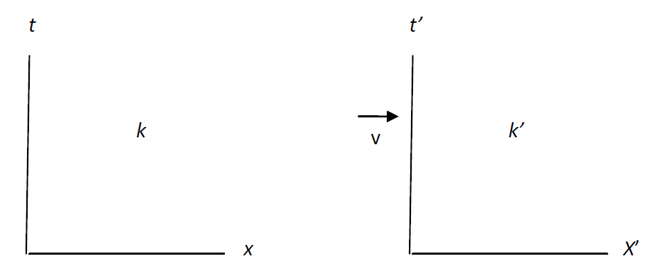
Coordinate system k′ moves uniformly with velocity v
relative to coordinate system k.
We consider two coordinate systems whose origins move with a constant velocity \(v\) relative to one another, respectively along the \(x\)- and \(x'\)-directions.
Although the coordinate systems are four-dimensional \((t, x, y, z)\), only the \(t\)- and \(x\)-axes are drawn for simplicity, since there is no motion in the \(y\)- and \(z\)-directions.
A light signal emitted at time \(t = t' = 0\) in the positive \(x\)-direction satisfies, in system \(k\):
\[ x = ct \quad\Rightarrow\quad x - ct = 0. \tag{1} \]
Since the same light signal also propagates with speed \(c\) in system \(k'\), we have:
\[ x' = ct' \quad\Rightarrow\quad x' - ct' = 0. \tag{2} \]
All spacetime points (events) that satisfy (1) must also satisfy (2). This is guaranteed if:
\[ x' - ct' = \lambda (x - ct), \tag{3} \]
where \(\lambda\) is a constant. If \(x - ct = 0\), then \(x' - ct' = 0\) automatically follows, independent of the value of \(\lambda\).
Light signal in the negative direction
For a light signal propagating along the negative \(x\)-axis, we have in \(k\):
\[ x + ct = 0, \]
and in \(k'\):
\[ x' + ct' = 0. \]
Therefore:
\[ x' + ct' = \mu (x + ct), \tag{4} \]
with \(\mu\) a second constant.
Linear combination of the two conditions
By adding and subtracting (3) and (4), and introducing the constants
\[ a = \frac{\lambda + \mu}{2}, \qquad b = \frac{\lambda - \mu}{2}, \]
we obtain:
\[ x' = a x - b c t, \qquad ct' = a ct - b x. \tag{5} \]
This is the general linear form of the Lorentz transformation, where the constants \(a\) and \(b\) still need to be determined.
Determination of the constant ratio \(b/a\)
For the origin of \(k'\) it holds permanently:
\[ x' = 0. \]
Substitution into the first equation of (5) gives:
\[ 0 = a x - b c t \quad\Rightarrow\quad x = \frac{b c}{a}\, t. \]
Thus, the origin of \(k'\) moves in \(k\) with velocity:
\[ v = \frac{b c}{a}. \tag{6} \]
This value \(v\) is the relative velocity of the two reference frames. The same value is obtained when calculating the velocity of any other point of \(k'\) with respect to \(k\), or vice versa.
The principle of relativity teaches us that — as judged from \(k\) — the length of a measuring rod at rest with respect to \(k'\) must be exactly equal to the length of a measuring rod at rest with respect to \(k\), as judged from \(k'\).
To see how the points on the \(x'\)-axis appear when viewed from \(k\), we take a snapshot of \(k'\) from \(k\). This means that we choose a fixed value of \(t\), for example:
\[ t = 0. \]
For this value, the first equation of (5) yields:
\[ x' = a x. \]
Two points on the \(x'\)-axis that are separated by a distance \(x' = L\) in \(k'\) are, in our snapshot, separated by:
\[ \Delta x = \frac{L}{a}. \tag{7} \]
Snapshot from \(k'\): \(t' = 0\)
If the snapshot is taken from \(k'\), that is at \(t' = 0\), then the second equation of (5) gives:
\[ 0 = a c t - b x \quad\Rightarrow\quad t = \frac{b}{a c} x. \]
Substitution into the first equation of (5) yields:
\[ x' = a x - b c t = a x - b c \left(\frac{b}{a c} x\right) = a x \left(1 - \frac{b^{2}}{a^{2}}\right). \]
From equation (6): \[ \frac{b}{a} = \frac{v}{c}, \] thus:
\[ x' = a \left(1 - \frac{v^{2}}{c^{2}}\right) x. \tag{7a} \]
Therefore, two points on the \(x\)-axis, separated by a distance \(L\) in \(k\), are represented in the snapshot from \(k'\) by:
\[ \Delta x' = a\left(1 - \frac{v^{2}}{c^{2}}\right) L. \tag{7b} \]
Equality of the two snapshots
According to the principle of relativity, both snapshots must be identical:
\[ \Delta x = \Delta x'. \]
Thus, according to equations (7) and (7b):
\[ \frac{L}{a} = a\left(1 - \frac{v^{2}}{c^{2}}\right) L. \]
After simplification:
\[ \frac{1}{a} = a\left(1 - \frac{v^{2}}{c^{2}}\right) \quad\Rightarrow\quad a^{2} = \frac{1}{1 - v^{2}/c^{2}}. \tag{7c} \]
Hence:
\[ a = \gamma = \frac{1}{\sqrt{1 - v^{2}/c^{2}}}, \qquad b = \gamma \frac{v}{c}. \]
The Lorentz transformation
By substituting these values of \(a\) and \(b\) into (5), we obtain:
\[ x' = a x - b c t = \gamma x - \gamma v t = \gamma (x - v t). \]
And:
\[ ct' = a c t - b x = \gamma c t - \gamma \frac{v}{c} x = \gamma\left(ct - \frac{v}{c} x\right). \]
Thus, the full Lorentz transformation reads:
\[ \boxed{ \begin{aligned} x' &= \gamma (x - vt), \\ t' &= \gamma\left(t - \frac{v}{c^{2}}x\right). \end{aligned} } \]
Lorentz transformation for events on the x-axis
From the previous derivation, the Lorentz transformation follows:
\[ x' = \frac{x - vt}{\sqrt{1 - v^{2}/c^{2}}}, \qquad t' = \frac{t - \frac{v}{c^{2}}x}{\sqrt{1 - v^{2}/c^{2}}}. \tag{8} \]
This transformation satisfies the invariance of the space–time interval:
\[ x'^{2} - c^{2}t'^{2} = x^{2} - c^{2}t^{2}. \tag{8a} \]
Extension to events off the x-axis
For motion exclusively along the x-axis, the transformations of the other coordinates remain unchanged:
\[ y' = y, \qquad z' = z. \tag{9} \]
With (8) and (9), we satisfy the postulate that the speed of light in vacuum has the same value in every inertial frame.
Verification using a light signal
A light signal emitted from the origin of \(k\) at time \(t = 0\) satisfies:
\[ r = \sqrt{x^{2} + y^{2} + z^{2}} = ct. \]
Squaring yields:
\[ x^{2} + y^{2} + z^{2} - c^{2}t^{2} = 0. \tag{10} \]
According to the principle of relativity, the same signal must satisfy in \(k'\):
\[ x'^{2} + y'^{2} + z'^{2} - c^{2}t'^{2} = 0. \tag{10a} \]
For (10a) to be a consequence of (10), it must hold that:
\[ x'^{2} + y'^{2} + z'^{2} - c^{2}t'^{2} = \zeta\, \left( x^{2} + y^{2} + z^{2} - c^{2}t^{2} \right). \tag{11} \]
But for points on the x-axis, equation (8a) already holds, hence:
\[ \zeta = 1. \]
This demonstrates that the Lorentz transformation (8)–(9) leaves the speed of light invariant.
General form of the Lorentz transformation
The Lorentz transformation derived above applies to the case in which:
- the axes of \(k\) and \(k'\) are parallel,
- the relative velocity \(v\) lies along the x-axis.
However, this is not a restriction. In general, any Lorentz transformation can be constructed from:
- a Lorentz transformation in the specific sense (translation along one axis),
- followed by a purely spatial rotation of the coordinate system.
This corresponds to replacing the rectangular coordinate system by a new one whose axes point in different directions.
In this way, we obtain the full Lorentz group, consisting of all combinations of translations and rotations.
The generalized Lorentz transformation
Mathematically, the generalized Lorentz transformation can be characterized as follows: it expresses \(x', y', z', t'\) in terms of linear homogeneous functions of \(x, y, z, t\), such that the relation
\[ x'^2 + y'^2 + z'^2 - c^2 t'^2 = x^2 + y^2 + z^2 - c^2 t^2 \tag{11a} \]
is satisfied identically. That is: when the expressions for \(x', y', z', t'\) in terms of \(x, y, z, t\) are substituted into the left-hand side, it becomes identically equal to the right-hand side.
Use of an imaginary time coordinate
We can characterize the Lorentz transformation even more simply by introducing the imaginary quantity \(i\), where \(i\) denotes \(\sqrt{-1}\). Define:
\[ x_1 = x,\qquad x_2 = y,\qquad x_3 = z,\qquad x_4 = i\,ct. \]
And analogously for the primed system \(k'\). Then the transformation condition becomes:
\[ x_1'^2 + x_2'^2 + x_3'^2 + x_4'^2 = x_1^2 + x_2^2 + x_3^2 + x_4^2. \tag{12} \]
With this choice of “coordinates”, equation (11a) is transformed into (12).
We see that the imaginary time coordinate \(x_4\) appears in the transformation condition in exactly the same way as the spatial coordinates \(x_1, x_2, x_3\). This reflects the relativistic insight that time and space are treated on equal footing in the laws of nature.
Minkowski space
A four-dimensional continuum described by the coordinates \((x_1, x_2, x_3, x_4)\) was called the world by Minkowski. A point-event is called a world point.
The four-dimensional “world” exhibits a strong analogy with three-dimensional Euclidean space. In Euclidean geometry, a rotation satisfies:
\[ x_1'^2 + x_2'^2 + x_3'^2 = x_1^2 + x_2^2 + x_3^2. \]
The analogy with (12) is complete: the Lorentz transformation corresponds to a “rotation” in four-dimensional Minkowski space, with the time coordinate carrying an imaginary component.
Appendix 9.2 — Alternative derivation of time dilation and length contraction
We now derive the relation between the time \(t\) in our coordinate system and the time \(t'\) in a system moving with velocity \(v\).
We take the origins of both systems to coincide at the instant:
\[ t = t' = 0. \]
As Einstein stated, the speed of light is the same in every inertial reference frame. Therefore, a light signal that moves with speed \(c\) in our system must also move with speed \(c\) in the moving system.
Time dilation via a light pulse perpendicular to the direction of motion
We consider a person in a rapidly moving object, for example a rocket, who emits a light pulse in a direction perpendicular to the direction of motion of the rocket.
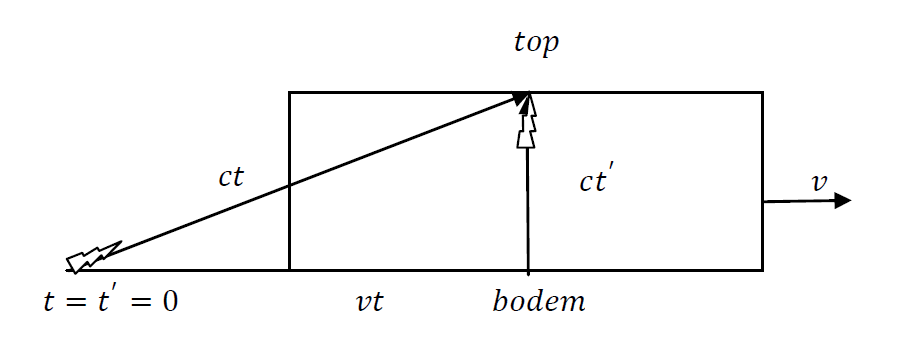
Time in our (stationary) system is denoted by \(t\), and time in the moving rocket by \(t'\).
In the rocket, the light pulse travels straight upward. The vertical distance covered in the rocket is:
\[ c t'. \]
From our stationary system, the rocket moves horizontally with velocity \(v\). Therefore, while the light pulse moves upward, it also moves horizontally.
We now compare the distances traveled in both systems.
In our system, the light pulse travels a diagonal distance:
\[ c t. \]
The horizontal displacement of the rocket (and thus of the light pulse) is:
\[ v t. \]
According to the Pythagorean theorem, we therefore have:
\[ c^{2} t^{2} = c^{2} t'^{2} + v^{2} t^{2}. \]
Rewriting yields:
\[ c^{2} t^{2} - v^{2} t^{2} = c^{2} t'^{2}, \] \[ t^{2}(c^{2} - v^{2}) = c^{2} t'^{2}, \] \[ t^{2}\left(1 - \frac{v^{2}}{c^{2}}\right) = t'^{2}. \]
Thus:
\[ \boxed{ t' = t \sqrt{1 - \frac{v^{2}}{c^{2}}} } \]
This shows that the time \(t'\) in the rocket is always shorter than the time \(t\) in our stationary system: time dilation.
Length contraction via a light pulse in the direction of motion
We now emit a light pulse in the horizontal direction, i.e. in the direction of motion.
Because the rocket moves horizontally, there is no vertical motion. The vertical direction is therefore unaffected by the velocity.
The horizontal direction is affected, because both the light pulse and the rocket move horizontally.
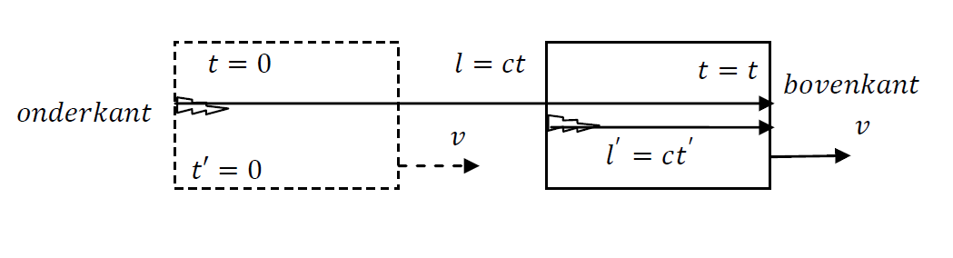
We consider the distance traveled by the pulse from the moment it starts at the left side of the rocket until it reaches the right side.
In our system, the distance traveled is:
\[ \ell = c t. \]
In the rocket, the distance traveled is:
\[ \ell' = c t'. \]
Since we previously found that:
\[ t' = t \sqrt{1 - \frac{v^{2}}{c^{2}}}, \]
it follows that:
\[ \ell' = c t' = c t \sqrt{1 - \frac{v^{2}}{c^{2}}} = \ell \sqrt{1 - \frac{v^{2}}{c^{2}}}. \]
Thus:
\[ \boxed{ \ell' = \ell \sqrt{1 - \frac{v^{2}}{c^{2}}} } \]
This shows that the length of an object moving with velocity \(v\) decreases in the direction of motion: length contraction.
Conclusion of time dilation and length contraction
The speed of light in our system is equal to the speed of light in the rocket, as observed from our point of view:
\[ c = \frac{\ell}{t} = \frac{\ell'}{t'}. \]
From the first part, we know that:
\[ t' = t \sqrt{1 - \frac{v^{2}}{c^{2}}}. \]
Therefore:
\[ \frac{\ell}{t} = \frac{\ell'}{t'} = \frac{\ell'}{t \sqrt{1 - v^{2}/c^{2}}}, \]
thus:
\[ \ell = \frac{\ell'}{\sqrt{1 - v^{2}/c^{2}}}, \qquad \ell' = \ell \sqrt{1 - \frac{v^{2}}{c^{2}}}. \]
The resulting relations are:
\[ \boxed{ t' = t \sqrt{1 - \frac{v^{2}}{c^{2}}} } \qquad\text{(time dilation)} \]
\[ \boxed{ \ell' = \ell \sqrt{1 - \frac{v^{2}}{c^{2}}} } \qquad\text{(length contraction)} \]
Thus, as observed from our reference frame, time in the rocket frame is shorter than our time, and the length of the rocket is shorter in the direction of motion.
Appendix 9.3 — Symmetry in the influence of spacetime under Lorentz transformations
Although the \(y\)- and \(z\)-coordinates themselves remain numerically constant, the time component \(t\) does change under the Lorentz transformation. As a result, processes that take place in the \(y\)- or \(z\)-direction evolve according to a modified time basis.
\[ x'=\gamma(x-vt) \] \[ t'=\gamma\left(t-\frac{v}{c^2}x\right) \] \[ y'=y \] \[ z'=z \]A clock located at a fixed \(y\)-position ticks more slowly for an observer at rest, exactly as a clock at a fixed \(x\)-position does. The same applies to events in the \(y\)-\(t\) or \(z\)-\(t\) plane: although the spatial component does not change, the time component is transformed.
Conversely, for the \(y\)-\(x\) and \(z\)-\(x\) planes: although the \(y\)- and \(z\)-coordinates remain constant, the \(x\)-coordinate changes under the Lorentz transformation. These planes are therefore also affected, although this influence is less directly visible in many applications.
This consideration leads to an important insight: the influence of a Lorentz transformation is not limited to the plane in which the velocity manifests itself (the \(x\)-\(t\) plane), but propagates structurally throughout the entire spacetime. Every plane in which one of the transformed coordinates \(x\) or \(t\) appears is partially determined by this transformation.
From this perspective, a form of structural symmetry emerges: even though \(y\) and \(z\) themselves do not change, processes in those directions still depend on a transformed time or space component. The entire spacetime is restructured, and with it all physical descriptions within that frame.
Appendix 9.4 — Trigonometric tools
Because trigonometric formulas are frequently used in special relativity, we provide a brief overview of several of them and how they can be easily derived.
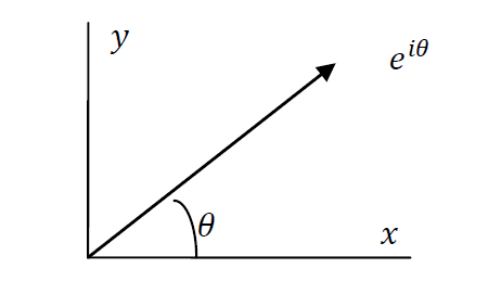
By definition:
\[ e^{i\theta} = \cos\theta + i\sin\theta \tag{1} \]
where: \[ i=\sqrt{-1} \]
Justification of this equation:
We first consider a function:
\[ F(x) = e^{\alpha x}. \]
Its derivative is:
\[ \frac{dF(x)}{dx} = \alpha F(x). \]
Thus, the derivative of an exponential function is the function itself multiplied by a factor \(\alpha\).
Complex trigonometric function
Now consider the function:
\[ F(x) = \cos(\alpha x) + i\sin(\alpha x). \]
Its derivative is:
\[ \frac{d}{dx}\left[\cos(\alpha x) + i\sin(\alpha x)\right] = -\alpha\sin(\alpha x) + i\alpha\cos(\alpha x) = i\alpha\left[\cos(\alpha x) + i\sin(\alpha x)\right]. \]
Thus:
\[ \frac{dF(x)}{dx} = i\alpha F(x). \]
From this it follows that:
\[ F(x) = e^{i\alpha x} = \cos(\alpha x) + i\sin(\alpha x). \]
For \(\alpha = 1\) we obtain the well-known Euler equation:
\[ \boxed{ e^{i\theta} = \cos\theta + i\sin\theta } \tag{1} \]
Derived trigonometric formulas
From (1) it follows directly that:
\[ e^{-i\theta} = \cos\theta - i\sin\theta. \tag{2} \]
By adding (1) and (2):
\[ \cos\theta = \frac{e^{i\theta} + e^{-i\theta}}{2}. \]
By subtracting (2) from (1):
\[ \sin\theta = \frac{e^{i\theta} - e^{-i\theta}}{2i}. \]
Furthermore:
\[ e^{i\theta} \cdot e^{-i\theta} = e^{i\theta - i\theta} = e^{0} = 1, \]
and:
\[ (\cos\theta + i\sin\theta)(\cos\theta - i\sin\theta) = \cos^{2}\theta + \sin^{2}\theta = 1. \]
Hyperbolic functions
We define:
\[ \cosh x = \frac{e^{x} + e^{-x}}{2}, \qquad \sinh x = \frac{e^{x} - e^{-x}}{2}. \]
From this it follows that:
\[ \cosh(x) = \cosh(-x), \qquad \sinh(x) = -\sinh(-x). \]
Furthermore:
\[ \cosh(ix) = \cos x, \qquad \sinh(ix) = i\sin x. \]
Thus:
\[ \boxed{ \cosh(ix) = \cos x,\qquad \sinh(ix) = i\sin x. } \]
These relations form the basis for the use of hyperbolic functions in special relativity, in particular in describing Lorentz boosts via rapidity.
Appendix 9.5 — Addition of velocities
We consider two coordinate systems \(A\) and \(B\) that move with a constant velocity \(v\) relative to each other. The axes are chosen such that the relative motion takes place along the \(x\)-axes.
In system \(A\), an object moves with velocity components \(V'_x, V'_y, V'_z\). We now wish to determine the velocity of this object relative to system \(B\).
According to Newton, the velocity in the \(x\)-direction would simply be: \[ V_x = V'_x + v. \] But according to special relativity, this is not correct.
Lorentz transformation
We begin with the Lorentz transformations:
\[ ct' = \gamma(ct - \beta x), \tag{1} \] \[ x' = \gamma(x - \beta ct), \tag{2} \] \[ y' = y,\qquad z' = z, \]
where: \[ \gamma = \frac{1}{\sqrt{1 - v^{2}/c^{2}}},\qquad \beta = \frac{v}{c}. \]
The inverse transformation is given by:
\[ ct = \gamma(ct' + \beta x'), \tag{1a} \] \[ x = \gamma(x' + \beta ct'), \tag{2a} \] \[ y = y',\qquad z = z'. \]
Velocity in the \(x'\)-direction
Take the derivative of (2):
\[ V'_x = \frac{dx'}{dt'} = \gamma\frac{dx}{dt}\frac{dt}{dt'} - \beta c \frac{dt}{dt'} = \gamma(V_x - \beta c)\frac{dt}{dt'}. \tag{3} \]
Now take the derivative of (1):
\[ c = \gamma\left(c\frac{dt}{dt'} - \beta \frac{dx}{dt}\frac{dt}{dt'}\right) = \gamma\left(c - \beta V_x\right)\frac{dt}{dt'}. \]
Thus:
\[ \frac{dt}{dt'} = \frac{1}{\gamma\left(1 - \beta\frac{V_x}{c}\right)}. \tag{4} \]
Substitute (4) into (3):
\[ V'_x = \gamma(V_x - \beta c) \cdot \frac{1}{\gamma\left(1 - \beta\frac{V_x}{c}\right)} = \frac{V_x - v}{1 - \frac{v V_x}{c^{2}}}. \tag{5} \]
This is the relativistic velocity addition formula in the \(x\)-direction.
Result
\[ \boxed{ V'_x = \frac{V_x - v}{1 - \frac{v V_x}{c^{2}}} } \]
This replaces the Newtonian addition \(V'_x = V_x - v\).
The velocities in the other directions are:
\[ V'_y = \frac{V_y}{\gamma\left(1 - \frac{v V_x}{c^{2}}\right)}, \qquad V'_z = \frac{V_z}{\gamma\left(1 - \frac{v V_x}{c^{2}}\right)}. \tag{6} \]
These formulas show that velocities do not simply add in relativity, but are influenced by both the Lorentz factor and the projection of the velocity along the direction of motion.
From equation (5) we already had:
\[ V'_x = \frac{\gamma(V_x - \beta c)}{\gamma\left(1 - \beta \frac{V_x}{c}\right)} = \frac{V_x - \beta c}{1 - \beta \frac{V_x}{c}} = \frac{V_x - v}{1 - \frac{v V_x}{c^{2}}}. \tag{5} \]
Velocity in the \(y'\)-direction
\[ V'_y = \frac{\partial y'}{\partial t'} = \frac{\partial y}{\partial t'} = \frac{\partial y}{\partial t}\frac{dt}{dt'} = V_y \frac{dt}{dt'}. \]
From equation (4):
\[ \frac{dt}{dt'} = \gamma\left(1 - \beta\frac{V_x}{c}\right), \]
thus:
\[ V'_y = \frac{V_y}{\gamma\left(1 - \beta\frac{V_x}{c}\right)}. \tag{6} \]
Velocity in the \(z'\)-direction
In an identical way one finds:
\[ V'_z = \frac{V_z}{\gamma\left(1 - \beta\frac{V_x}{c}\right)}. \tag{7} \]
Interpretation of equation (4)
From (4):
\[ \frac{dt}{dt'} = \frac{1}{\gamma\left(1 - \beta\frac{V_x}{c}\right)} = \frac{1 - v^{2}/c^{2}}{1 - \frac{v V_x}{c^{2}}}. \]
In the special case where \(V'_x = 0\), we have \(V_x = v\). Then:
\[ \frac{dt}{dt'} = \frac{1 - v^{2}/c^{2}}{1 - v^{2}/c^{2}} = \frac{1}{1 - v^{2}/c^{2}} = \gamma^{2}. \]
Thus:
\[ dt' = \sqrt{1 - \frac{v^{2}}{c^{2}}}\, dt, \]
and therefore:
\[ dt' \ll dt. \]
This is again time dilation.
Back to the general case
From (5):
\[ V'_x = \frac{V_x - v}{1 - \frac{v V_x}{c^{2}}}. \]
Solving for \(V_x\) gives:
\[ V_x = \frac{V'_x + v}{1 + \frac{v V'_x}{c^{2}}}. \]
This is the inverse relativistic velocity addition.
In compact form:
\[ \boxed{ V_x = \frac{V'_x + v}{1 + \beta \frac{V'_x}{c}} } \tag{5a} \]
For the other components one analogously finds:
\[ V_y = \frac{V'_y}{\gamma\left(1 + \beta\frac{V'_x}{c}\right)}, \tag{6a} \]
and:
\[ V_z = \frac{V'_z}{\gamma\left(1 + \beta\frac{V'_x}{c}\right)}. \tag{7a} \]
Summary
The relativistic velocity addition formulas are:
\[ \boxed{ V'_x = \frac{V_x - v}{1 - \frac{v V_x}{c^{2}}} } \]
\[ \boxed{ V'_y = \frac{V_y}{\gamma\left(1 - \frac{v V_x}{c^{2}}\right)} } \]
\[ \boxed{ V'_z = \frac{V_z}{\gamma\left(1 - \frac{v V_x}{c^{2}}\right)} } \]
and the inverse transformation:
\[ \boxed{ V_x = \frac{V'_x + v}{1 + \frac{v V'_x}{c^{2}}} } \]
\[ \boxed{ V_y = \frac{V'_y}{\gamma\left(1 + \frac{v V'_x}{c^{2}}\right)} } \]
\[ \boxed{ V_z = \frac{V'_z}{\gamma\left(1 + \frac{v V'_x}{c^{2}}\right)} } \]
For the \(z\)-component one similarly obtains:
\[ V'_z = \frac{V_z}{\gamma\left(1 + \beta \frac{V'_x}{c}\right)}. \tag{7a} \]
According to Newton one would simply add velocities in the \(x\)-direction:
\[ V_x = V'_x + v. \]
But according to special relativity this is corrected to:
\[ V_x = \frac{V'_x + v}{1 + \frac{v V'_x}{c^{2}}}. \]
In general, when the term \(\frac{v V'_x}{c^{2}}\) is very small, the relativistic result can be approximated by the Newtonian one:
\[ V_x \approx V'_x + v. \]
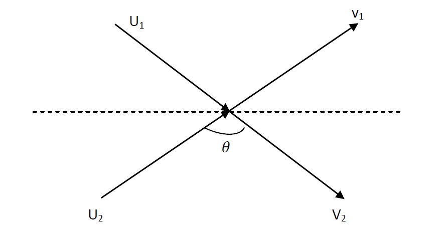
Appendix 9.6 Collisions
Consider a perfectly elastic collision between two identical particles; an elastic collision is a collision without loss of kinetic energy. The initial velocities of the particles are respectively \(\vec{u_1}\) and \(\vec{u_2}\), and after the collision \(\vec{v_1}\) and \(\vec{v_2}\). Due to conservation of momentum we have: \[ m_{1u}u_1+m_{2u}u_2=m_{1v}v_1+m_{2v}v_2 \] Here \(m_{1u}\) and \(m_{2u}\) are the masses before the collision, and \(m_{1v}\) and \(m_{2v}\) the masses after the collision.
First we consider the collision from a coordinate system moving with particle one. Then particle 1 moves upward with velocity \(w_1\) and downward with \(w_2\). These velocities are equal in magnitude but opposite in direction. Particle 2 has velocity \(V\) with an \(x\)-component \(u\) and a \(y\)-component \(v\).
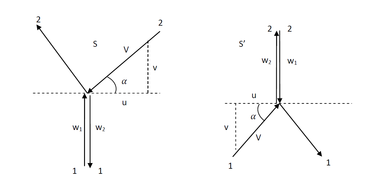
Left: Collision between two identical particles in a coordinate system S moving with particle 1. Right: The same, but now in S′ moving with particle 2.
Relation between the y-components of the momentum
We now want to find the relation between the y-components of the momentum of particles 1 and 2 in system \(S\), i.e. between \(w\) and \(v\).
In the previous chapter we found the relation:
\[ V'_y = \frac{V_y}{\gamma\left(1 - \beta \frac{V_x}{c}\right)}. \]
Since in this case: \[ V_y = w,\qquad V_x = 0, \] we obtain:
\[ v = \frac{w}{\gamma} \]
Due to symmetry, \(w\) is the velocity of particle 1 in system \(S\) and the velocity of particle 2 in system \(S'\). Conversely, \(v\) is the y-component of particle 2 in \(S\) and of particle 1 in \(S'\).
Total velocity
The total velocity of the moving particle in \(S\) and in \(S'\) is the same:
\[ V = \sqrt{v^{2} + u^{2}}. \]
Conservation of momentum in the y-direction
Momentum conservation in the y-direction gives:
\[ m_w w - m_V v = -m_w w + m_V v. \]
From this it follows that:
\[ m_w w = m_V v. \]
Thus:
\[ \frac{m_V}{m_w} = \frac{w}{v} = \frac{w}{w/\gamma} = \gamma. \tag{1} \]
This result shows that the Lorentz factor \(\gamma\) arises directly from momentum conservation in a collision that is viewed symmetrically from two inertial frames.
Low-velocity limit
Now suppose that the velocity \(w\) is very small. In this limit we have:
\[ \lim_{w \to 0} v = 0, \qquad \lim_{w \to 0} V = u. \]
In this case relativistic effects can be neglected and the classical expression for momentum is recovered.
Since: \[ \lim_{w \to 0} m_w = m, \] we substitute this into equation (1):
\[ \lim_{w \to 0} m_V = \gamma m = \frac{m}{\sqrt{1 - \frac{u^{2}}{c^{2}}}}. \]
Because of momentum conservation, the definition of momentum must be modified. The relativistic momentum therefore becomes:
\[ \boxed{ \vec{p} = \gamma m \vec{v} } \]
Appendix 9.7 — The Energy of a Moving Object
Using a thought experiment, Einstein demonstrated that energy and mass are equivalent via the relation \(E = mc^2\). We have shown that for an object moving with velocity, the momentum must be adapted to the relativistic description: \[ \vec{p} = \gamma m \vec{v} \] It can therefore be stated that the energy of an object is equal to: \[ E = \gamma m c^2 \] Thus: \[ E = \frac{mc^2}{\sqrt{1 - \frac{u^2}{c^2}}} \] Using the Taylor series expansion: \[ E = \gamma m c^2 \approx mc^2\left(1+\frac{v^2}{2c^2}-\frac{3v^4}{8c^4}\text{.....} \right) \]
If \(v\) is much smaller than \(c\), the third and higher-order terms inside the parentheses can be neglected. This leads to:
\[ E \approx mc^2 + \frac{1}{2}mv^2 \]
Thus this is the kinetic energy \(\frac{1}{2}mv^2\) plus a constant \(mc^2\).
Appendix 9.8 — Energy-Momentum Vector
As found by Minkowski, the spacetime interval is:
\[ c^{2} d\tau^{2} = c^{2} dt^{2} - dx^{2} - dy^{2} - dz^{2}. \tag{1} \]
We write this as:
\[ c^{2} d\tau^{2} = c^{2} dt^{2} \left( 1 - \frac{dx^{2} + dy^{2} + dz^{2}}{c^{2} dt^{2}} \right) = c^2dt^{2}\left(1 - \frac{v^{2}}{c^{2}}\right). \]
Since: \[ \gamma = \frac{1}{\sqrt{1 - v^{2}/c^{2}}}, \] it follows that:
\[ 1 - \frac{v^{2}}{c^{2}} = \frac{1}{\gamma^{2}}, \qquad d\tau^{2} = \frac{dt^{2}}{\gamma^{2}}, \qquad \gamma = \frac{dt}{d\tau}. \]
Derivation of the Energy–Momentum Relation
Begin again from (1):
\[ c^{2} = c^{2}\left(\frac{dt}{d\tau}\right)^{2} - \left(\frac{dx}{dt}\right)^{2}\left(\frac{dt}{d\tau}\right)^{2} - \left(\frac{dy}{dt}\right)^{2}\left(\frac{dt}{d\tau}\right)^{2} - \left(\frac{dz}{dt}\right)^{2}\left(\frac{dt}{d\tau}\right)^{2} \]
Multiply by the rest mass \(m_{0}^{2}\):
\[ m_{0}^{2} c^{2} = m_{0}^{2} c^{2}\left(\frac{dt}{d\tau}\right)^{2} - m_{0}^{2}\left(\frac{dx}{dt}\right)^{2}\left(\frac{dt}{d\tau}\right)^{2} - m_{0}^{2}\left(\frac{dy}{dt}\right)^{2}\left(\frac{dt}{d\tau}\right)^{2} - m_{0}^{2}\left(\frac{dz}{dt}\right)^{2}\left(\frac{dt}{d\tau}\right)^{2} \]
Since: \[ \frac{dt}{d\tau} = \gamma, \] we obtain:
\[ m_{0}^{2} c^{2} = \gamma^{2} m_{0}^{2} c^{2} - \gamma^{2} m_{0}^{2} v_x^{2} - \gamma^{2} m_{0}^{2} v_y^{2} - \gamma^{2} m_{0}^{2} v_z^{2}. \]
Now define the four-momentum:
\[ p_{0} = \frac{E}{c}, \qquad p_{1} = p_x, \qquad p_{2} = p_y, \qquad p_{3} = p_z, \]
with: \[ p_i = \gamma m_0 v_i. \]
Then the Minkowski norm becomes:
\[ p_{\tau}^{2} = \left(\frac{E}{c}\right)^{2} - p_x^{2} - p_y^{2} - p_z^{2} = m_{0}^{2} c^{2}. \]
Or more compactly:
\[ E^{2} - c^{2} |\vec{p}|^{2} = m_{0}^{2} c^{4}. \]
Thus:
\[ \boxed{ E^{2} = m_{0}^{2} c^{4} + c^{2} p^{2} } \]
and for positive energy:
\[ \boxed{ E = +\sqrt{m_{0}^{2} c^{4} + c^{2} p^{2}}. } \]
We found that: \[ p = \gamma m_0 v = \frac{m_0 v}{\sqrt{1 - \frac{v^{2}}{c^{2}}}}, \] where \(m_0\) is the rest mass (the mass at zero velocity).
From the relation: \[ E = \frac{m_0 c^{2}}{\sqrt{1 - \frac{v^{2}}{c^{2}}}} \] it follows that:
\[ E^{2} = \frac{m_0^{2} c^{4}}{1 - \frac{v^{2}}{c^{2}}}. \]
After further rearranging:
\[ E^{2} = m_0^{2} c^{4} + \frac{m_0^{2} c^{4} \frac{v^{2}}{c^{2}}}{1 - \frac{v^{2}}{c^{2}}} = m_0^{2} c^{4} + \frac{m_0^{2} v^{2} c^{2}}{1 - \frac{v^{2}}{c^{2}}}. \]
But: \[ p = \frac{m_0 v}{\sqrt{1 - \frac{v^{2}}{c^{2}}}} \quad\Rightarrow\quad p^{2} = \frac{m_0^{2} v^{2}}{1 - \frac{v^{2}}{c^{2}}}. \]
Thus:
\[ E^{2} = m_0^{2} c^{4} + p^{2} c^{2}. \]
Or as commonly written:
\[ \boxed{ E^{2} = p^{2} c^{2} + m_{0}^{2} c^{4} } \tag{2} \]
where: \[ p = \frac{m_0 v}{\sqrt{1 - \frac{v^{2}}{c^{2}}}}. \]
Appendix 9.8.1 Alternative Derivation of the Energy–Momentum–Mass Relation
We had: \[ p = m v \] \[ p = \gamma m_0 v = \gamma m_0 c^2 \frac{v}{c^2} \]
\[ p c = \gamma m_0 c^2 \frac{v}{c} = \beta \gamma m_0 c^2 \]
Here: \[ \gamma = \frac{1}{\sqrt{1 - \beta^2}} \quad \text{and} \quad \beta = \frac{v}{c}. \]
Now, using the above, we examine what happens:
\[ ( p c )^2 + ( m_0 c^2 )^2 = ( \beta \gamma m_0 c^2 )^2 + ( m_0 c^2 )^2 \]
\[ = ( m_0 c^2 )^2 ( \beta^2 \gamma^2 + 1 ) \]
\[ = ( m_0 c^2 )^2 \left( 1 + \frac{\beta^2}{1 - \beta^2} \right) \]
\[ = ( m_0 c^2 )^2 \gamma^2 \]
\[ = ( \gamma m_0 c^2 )^2 = E^2 \]
Thus:
\[ \boxed{ E^{2} = p^{2} c^{2} + m_{0}^{2} c^{4} } \]
Appendix 9.8.2 — Classical Proof of Energy Conservation
The total mechanical energy of a particle is the sum of the kinetic energy \(K\) and the potential energy \(U\):
\[ E = \frac{1}{2} m v^{2} + U(x). \]
Taking the time derivative (one-dimensional motion):
\[ \frac{dE}{dt} = m v \frac{dv}{dt} + \frac{dU}{dx} \frac{dx}{dt} = m v a + v \frac{dU}{dx}. \]
The force corresponding to a potential energy \(U(x)\) is:
\[ F = -\frac{dU}{dx}. \]
Thus:
\[ \frac{dE}{dt} = v ( m a - F ). \]
According to Newton’s second law:
\[ F = m a. \]
Therefore:
\[ \frac{dE}{dt} = 0. \]
Hence:
\[ \boxed{E = \text{constant}} \]
The total mechanical energy is therefore conserved.
Appendix 9.9 Derivation of \(E = m c^2\)
Einstein’s Thought Experiment with the Light Pulse in a Box
Einstein derived the equation \(E = m c^{2}\) by means of an elegant thought experiment. Consider a stationary box freely floating in space, without gravity or external forces.
At the left side of the box, a photon is emitted and travels to the right. By conservation of momentum, the box moves slightly to the left. When the photon reaches the right wall, it transfers its entire momentum to the box, causing the box to come to rest again.
The photon has moved, and the box has also moved, but no external forces are present. Therefore, the center of mass of the total system must remain constant.
Relativistic Energy of the Photon
From Appendix 9.6 (equation (2)) we know:
\[ E^{2} = p^{2} c^{2} + m_{0}^{2} c^{4}. \]
For a photon we have \(m_{0} = 0\), hence:
\[ E = p c. \]
The momentum of the photon is therefore: \[ p_{\text{photon}} = \frac{E}{c}. \]
Momentum of the Box
The box with mass \(M\) moves slightly to the left with velocity \(v\). The momentum of the box is:
\[ p_{\text{box}} = M v. \]
During the time \(\Delta t\) that the photon needs to reach the right side, the box is displaced over a distance \(\Delta x\). The velocity of the box is therefore:
\[ v = -\frac{\Delta x}{\Delta t}. \]
Due to conservation of momentum: \[ p_{\text{photon}} + p_{\text{box}} = 0 \quad\Rightarrow\quad p_{\text{box}} = -p_{\text{photon}}. \]
Thus:
\[ M \frac{\Delta x}{\Delta t} = \frac{E}{c}. \]
The length of the box is \(L\), so the time required for the photon to reach the other side is:
\[ \Delta t = \frac{L}{c}. \]
Hence:
\[ M \Delta x = \frac{E L}{c^{2}}. \]
Center of Mass of the System
Now suppose hypothetically that the photon has a small mass \(m\). Then we can determine the center of mass of the system. If the position of the box is \(x_{1}\) and the position of the photon is \(x_{2}\), the center of mass is:
\[ \bar{x} = \frac{M x_{1} + m x_{2}}{M + m}. \]
Since no external forces act on the system, this center of mass must remain constant:
\[ \frac{M x_1 + m x_2}{M + m} = \frac{M(x_1 - \Delta x) + m L}{M + m}. \]
The photon starts at \(x_2 = 0\), so we obtain:
\[ m L = M \Delta x. \]
Using the earlier result:
\[ m L = \frac{E L}{c^{2}}. \]
With some rearrangement we obtain the famous relation:
\[ \boxed{ E = m c^{2}. } \]
Remark — Accurate Treatment of the Photon Path
In the original derivation it is assumed that the photon travels a distance L. In reality, however, the box moves a small distance \(\Delta x\) in the opposite direction during the flight of the photon. The effective photon path is therefore:
\[ L\sqrt{1 - \frac{v^{2}}{c^{2}}} - \Delta x. \]
This leads to a modified travel time:
\[ \Delta t = \frac{L\sqrt{1 - \frac{v^{2}}{c^{2}}} - \Delta x}{c}. \]
Momentum balance gives:
\[ M\,\frac{\Delta x}{\Delta t} = \frac{E}{c} \quad\Rightarrow\quad M\Delta x = \frac{E}{c}\,\Delta t. \]
Substituting \(\Delta t\) yields:
\[ M\Delta x = \frac{E}{c^{2}} \left( L\sqrt{1 - \frac{v^{2}}{c^{2}}} - \Delta x \right). \]
Center-of-Mass Condition
The center of mass of the box + photon system must remain constant:
\[ \frac{M x_{1} + m x_{2}}{M + m} = \frac{M(x_{1} - \Delta x) + m\left(L\sqrt{1 - \frac{v^{2}}{c^{2}}} - \Delta x\right)} {M + m}. \]
This yields:
\[ - M\Delta x + m\left(L\sqrt{1 - \frac{v^{2}}{c^{2}}} - \Delta x\right) = 0. \]
Thus:
\[ m\left(L\sqrt{1 - \frac{v^{2}}{c^{2}}} - \Delta x\right) = M\Delta x. \]
But earlier we found:
\[ M\Delta x = \frac{E}{c^{2}} \left( L\sqrt{1 - \frac{v^{2}}{c^{2}}} - \Delta x \right). \]
Therefore:
\[ \frac{E}{c^{2}} \left( L\sqrt{1 - \frac{v^{2}}{c^{2}}} - \Delta x \right) = m\left( L\sqrt{1 - \frac{v^{2}}{c^{2}}} - \Delta x \right). \]
Since the factor in parentheses is nonzero, we obtain:
\[ \boxed{E = m c^{2}}. \]
Conclusion
Even when we:
- take the displacement of the box \(\Delta x\) into account,
- use the shortened photon path,
- include Lorentz contraction,
the derivation still leads exactly to:
\[ \boxed{E = m c^{2}}. \]
Appendix 9.10 — Applications
Appendix 9.10.1 — Nuclear Fusion and Fission
When a proton \(p\) and a neutron \(n\) are brought together, they may fuse into a deuterium nucleus \(d\). The masses of the particles involved are:
\[ m_{p} = 938.27231\ \text{MeV}/c^{2},\qquad m_{n} = 939.56563\ \text{MeV}/c^{2},\qquad m_{d} = 1875.61339\ \text{MeV}/c^{2}. \]
Unit: MeV/\(c^{2}\)
From the relation \(E = m c^{2}\) it follows that mass can be expressed as energy divided by \(c^{2}\). In particle physics, the electronvolt (eV) is therefore commonly used:
\[ 1\ \text{eV} = 1.6\times 10^{-19}\ \text{J},\qquad 1\ \text{MeV} = 10^{6}\ \text{eV}. \]
The unit MeV/\(c^{2}\) is therefore a practical measure of mass.
Released Energy in Fusion
Since the mass of the deuteron is smaller than the sum of the masses of the proton and neutron, energy must have been released. If \(p\) and \(n\) combine with negligible initial velocity:
\[ E = m_{p} c^{2} + m_{n} c^{2} - m_{d} c^{2} = 2.22455\ \text{MeV}. \]
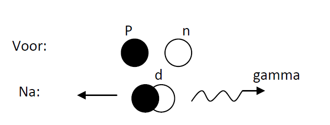
This energy is released in the form of a photon:
\[ p + n \;\rightarrow\; d + \gamma. \]
A photon is massless and carries energy and momentum. To ensure momentum conservation, the deuteron moves in the opposite direction of the photon. Because the mass of \(d\) is large, its kinetic energy is very small:
\[ E = \sqrt{p^{2} c^{2} + m^{2} c^{4}} \approx m c^{2} \qquad\text{when }\quad p c \ll m c^{2}. \]
Nuclear Fusion
The reaction described above is an example of nuclear fusion. Light nuclei can fuse into heavier nuclei while releasing energy. All nuclei up to iron (\(^{56}\text{Fe}\)) can be formed by fusion with net energy production.
Nuclear Fission
For very heavy nuclei, such as uranium, the opposite holds: the total mass of the nucleus is greater than the sum of the masses of the individual nucleons. Energy is therefore released when such heavy nuclei split:
nuclear fission.
This explains why:
- fusion releases energy for light elements,
- fission releases energy for heavy elements.
Appendix 9.10.2 — Driving an Electric Car on 1 Gram of Hydrogen via Nuclear Fusion
Here we examine how much energy is released in the nuclear fusion of hydrogen as in the Sun, where four hydrogen atoms fuse into one helium atom. A small part of the mass disappears and is converted into energy according to \(E = mc^{2}\). We then determine how many kilometers an electric car could theoretically drive using this energy.
1. Energy Yield from Nuclear Fusion
Fusion in the Sun occurs via the proton-proton chain. The net reaction is:
\[ 4\,{}^{1}_1\!H \;\rightarrow\; {}^{4}_2\!He + 2e^{+} + 2\nu_{e} + 2\gamma. \]
The mass of four hydrogen atoms is larger than that of one helium nucleus. The mass difference is released as energy. Per fusion of four hydrogen atoms, approximately:
\[ 26.7\ \text{MeV} \]
is released.In 1 gram of hydrogen there are approximately \(6.022\times 10^{23}\) (Avogadro's number) hydrogen atoms (1 mol). Thus, in 1 gram of hydrogen, we have \[\frac{6.022 \times 10^{23}}{4} \approx 1.505 \times 10^{23}\] fusion reactions.
Each fusion reaction gives 26.7 MeV of energy, so the total energy is:
\[ E_{\text{fusion}} = 1.505\times 10^{23} \times 26.7\ \text{MeV}. \]
2. Conversion from MeV to Joule
One Joule equals the work done in moving a charge of 1 Coulomb through a potential of 1 Volt. Thus \[Joule = qV\].
The charge of an electron \(e\) is \(1.60218 \times 10^{-19}\, \text{C}\).
Then:
\[ 1\ \text{eV} = 1.60218\times 10^{-19}\ \text{J}, \qquad 1\ \text{MeV} = 1.60218\times 10^{-13}\ \text{J}. \]
Thus, for 1 gram of hydrogen, the total energy in Joules is:
\[ E_{\text{total}} = 1.505\times 10^{23} \times 26.7 \times 1.60218\times 10^{-13} \approx 6.43\times 10^{11}\ \text{J}. \]
3. Calculation of the Energy
\[ E_{\text{total}} \approx 6.43\times 10^{11}\ \text{Joules per gram of hydrogen}. \]
This is the energy released in this process, where a small portion of the mass
is converted into energy.
For comparison, consider the theoretical calculation if 1 gram of matter were completely
converted according to \(E=mc^2\):
\[
E = \frac{1}{1000} \times (3\times 10^8)^2 \approx 9 \times 10^{13}\ \text{J}.
\]
Thus, fusion releases roughly a factor 140 less energy (or about 0.7% of the energy from
complete conversion of 1 gram of mass).
4. Alternative Mass Defect Calculation
In fusion, 4 mol of hydrogen are converted into 1 mol of helium:
\[ m_{H,4} = 4 \times 1.00784 = 4.03136\ \text{g}, \qquad m_{He} = 4.0026\ \text{g}. \]
Mass difference:
\[ \Delta m = 0.02876\ \text{g} = 2.876 \times 10^{-5}\ \text{kg}. \]
Energy released:
\[ E = \Delta m\,c^{2} = 2.876\times 10^{-5} (3\times 10^{8})^{2} \approx 2.588\times 10^{12}\ \text{J} \]
for 4.03136 g of hydrogen, so: \[ E \approx 6.42\times 10^{11}\ \text{J per gram}. \]
5. Energy Consumption of an Electric Car
Electric cars consume on average:
\[ 17\ \text{kWh per 100 km}. \] \[ 1\ \text{kWh} = 3.6\times 10^{6}\ \text{J}, \qquad 17\ \text{kWh} = 61.2\times 10^{6}\ \text{J per 100 km}. \]
6. Theoretical Driving Distance (100% Efficiency)
\[ \text{Distance} = \frac{6.43\times 10^{11}}{61.2\times 10^{6}} \times 100\ \text{km} \approx 1.05\times 10^{6}\ \text{km}. \]
7. Realistic Efficiency
- Fusion → electricity efficiency: 40%
- Electric drivetrain efficiency: 90%
Total efficiency:
\[ \eta = 0.4 \times 0.9 = 0.36. \]
Usable energy:
\[ E_{\text{usable}} = 6.43\times 10^{11} \times 0.36 = 2.31\times 10^{11}\ \text{J}. \]
8. Practical Driving Distance
\[ \text{Distance} = \frac{2.31\times 10^{11}}{61.2\times 10^{6}} \times 100\ \text{km} \approx 3.77\times 10^{5}\ \text{km}. \]
Thus, an electric car could theoretically drive:
\[ \boxed{ \text{approximately } 3.77\times 10^{5}\ \text{km} } \]
on the energy from nuclear fusion of 1 gram of hydrogen.
At an average annual mileage of 15,000 km, this corresponds to:
\[ \frac{3.77\times 10^{5}}{1.5\times 10^{4}} \approx 25\ \text{years}. \]
In other words: 1 gram of hydrogen could theoretically power electric driving for about 25 years.
Appendix 9.11 — Relativistic Electromagnetism
(Calculations based on Richard Feynman, Feynman Lectures on Physics, Vol. II, Chapter 13)
Appendix 9.11.1 — Introduction
The word electromagnetism suggests that there are two types of fields: an electric field and a magnetic field, each with its own sources. In reality, we know only one fundamental source: electric charge.
Electric charges — electrons with charge \(-e\) and protons with charge \(+e\) — are the only known sources of the electric field. To date, no magnetic monopoles have been found that could serve as sources of a magnetic field.
It strongly appears that magnetic fields always arise from:
- moving electric charges (currents), or
- time variations of the electric field.
Even at the quantum scale, magnetic fields result from electric phenomena, such as the spins of electrons and atoms.
Therefore, the magnetic field model is an extremely useful mathematical tool to describe electromagnetic phenomena, but the underlying physical phenomenon is entirely electric in nature: an electric field and its variation in space and time.
Appendix 9.11.2 — Calculations
When analyzing a current-carrying wire, we normally use the Maxwell equations to determine both the electric and magnetic fields.
An alternative — and in a relativistic context very insightful — approach is to perform the full calculation using only the electric field, and to consider the magnetic field as a relativistic byproduct.
This idea forms the core of Feynman's treatment of electromagnetism: the magnetic field is what an electric field looks like when viewed from another inertial frame.
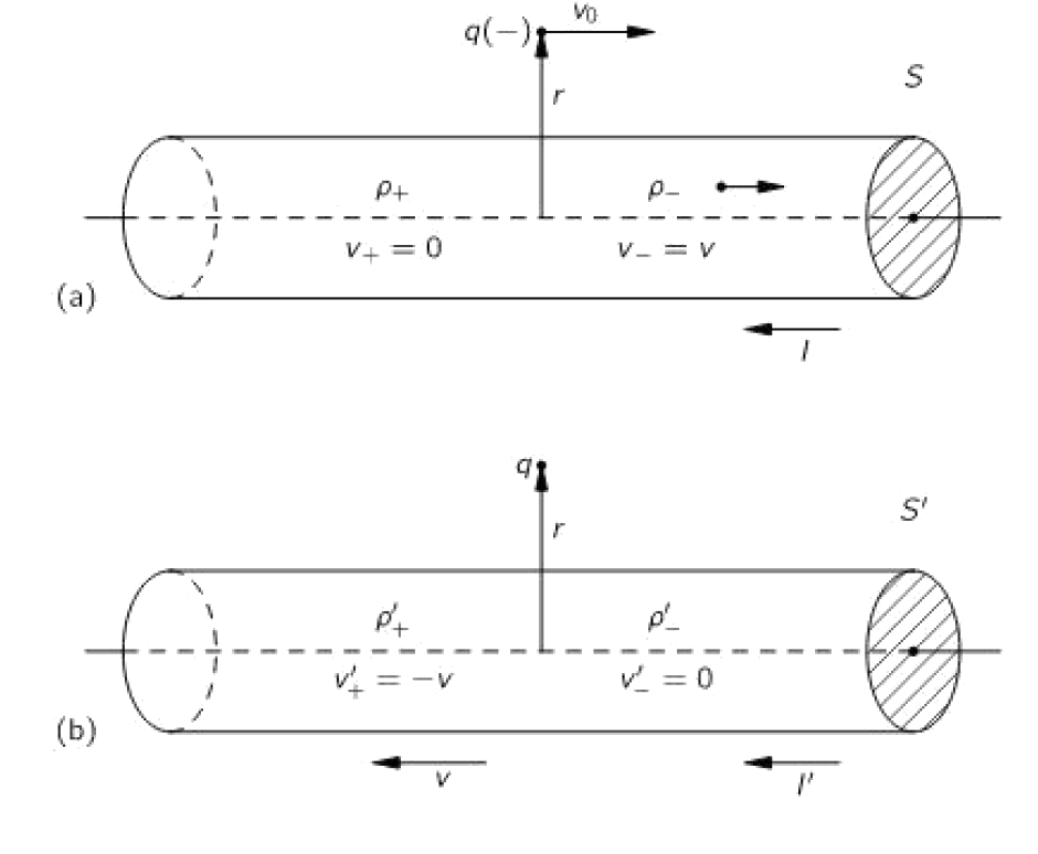
We consider a wire carrying electric current and a test charge \(q\). The situation is viewed in two different inertial frames:
- Frame S — the wire is at rest, the charge moves.
- Frame S′ — the charge is at rest, the wire moves.
Although the physical situation is the same, the fields in the two frames are observed differently. This is exactly where relativity and electromagnetism meet.
In the following sections, we will derive some fundamental formulas showing how electric fields and charge densities transform under Lorentz transformations, and how the magnetic field automatically follows from this.
Current density and charge distribution
The current density is the average flow velocity of the charges. Assume there is a distribution of charges with an average velocity \(\vec{v}\). The charge \(\Delta q\) that passes through a surface element \(\Delta S\) during a time interval \(\Delta t\) is:
\[ \Delta q = \rho\, \vec{v}\cdot\vec{n}\, \Delta S\, \Delta t. \tag{1} \]
Here, \(\rho\) is the charge density: the charge per unit volume. The term \(\vec{v}\Delta t \cdot \Delta S\) can be interpreted as a volume. Thus, the charge is the charge density times the volume.
The charge per unit time is then: \[ \rho\, \vec{v}\cdot\vec{n}\, \Delta S. \]
Therefore, we define the current density:
\[ \boxed{\vec{j} = \rho\, \vec{v}} \tag{2} \]
The total current through a surface \(S\) is:
\[ i = \int_{S} \vec{j}\cdot d\vec{S}. \tag{3} \]
Current carrier at rest
We now consider a wire that is at rest. The electrons (negative charges) move to the right with velocity \(v\). The protons (positive charges) remain at rest in the wire.
A test particle with negative charge \(q^{-}\) moves with the same velocity as the electrons to the right. We observe everything in the frame in which the wire is at rest.
The wire is electrically neutral: \[ \rho_{+} + \rho_{-} = 0. \]
Force on the test particle
The force on a charge is given by the Lorentz force:
\[ \vec{F} = q(\vec{E} + \vec{v} \times \vec{B}). \]
The magnetic field around a long straight wire is:
\[ H = \frac{i}{2\pi r}, \qquad B = \mu_{0} H. \]
Since the wire is neutral, the electric field outside the wire is zero: \[ \vec{E} = 0. \]
The force on the test particle then becomes:
\[ F = q\, v B \sin\varphi. \]
Since \(\vec{v}\) is perpendicular to \(\vec{B}\), \(\sin\varphi = 1\), so:
\[ F = q v B = q v \mu_{0} H = q v \mu_{0} \frac{i}{2\pi r}. \]
Charge density
The charge density is defined as:
\[ \rho = \frac{q}{V}. \]
If \(A\) is the cross-sectional area of the wire and \(L\) is any length along the wire, then the volume is: \[ V = A L, \] and thus: \[ q = \rho A L. \]
When the wire is at rest, we have: \[ \rho_{+} + \rho_{-} = 0. \]
This forms the basis for the relativistic analysis that follows: in one frame the wire is neutral, but in another frame — due to Lorentz contraction — the charge density changes, producing an electric field that exactly corresponds to the magnetic effect in the original frame.
Relativistic consideration from the perspective of the test particle
We now examine the situation from the frame in which the test particle is at rest. In this frame, the wire moves to the left with velocity \(v\). The volume is determined by the cross-section \(A\) and length \(L\).
The length of a moving volume relative to a volume at rest is: \[ L_{\text{moving}} = L_{\text{rest}} \sqrt{1 - \frac{v^{2}}{c^{2}}}. \]
Since the electrons have the same velocity as the test particle, they are at rest in this frame. Thus: \[ L_{\text{rest}} = \frac{L_{\text{moving}}}{\sqrt{1 - \frac{v^{2}}{c^{2}}}}. \]
The positive ions now move to the left with velocity \(v\). Their length is Lorentz-contracted by the factor: \[ \frac{1}{\sqrt{1 - \frac{v^{2}}{c^{2}}}}. \]
New charge density
In the rest frame of the wire, the external electric field was zero: \[ \rho_{+} + \rho_{-} = 0. \]
But in the frame of the test particle, the moving length is smaller, so the moving volume is smaller, and thus the charge density is higher.
The charge density of the electrons is therefore: \[ \rho_{-}' = \rho_{-} \sqrt{1 - \frac{v^{2}}{c^{2}}}. \]
The positive charge density becomes: \[ \rho_{+}' = \frac{\rho_{+}}{\sqrt{1 - \frac{v^{2}}{c^{2}}}}. \]
The total charge density is then: \[ \rho_{\text{net}} = \rho_{+}' + \rho_{-}' = \frac{\rho_{+}}{\sqrt{1 - \frac{v^{2}}{c^{2}}}} + \rho_{-} \sqrt{1 - \frac{v^{2}}{c^{2}}}. \]
Since \(\rho_{-} = -\rho_{+}\):
\[ \rho_{\text{net}} = \rho_{+} \left( \frac{1}{\sqrt{1 - \frac{v^{2}}{c^{2}}}} - \sqrt{1 - \frac{v^{2}}{c^{2}}} \right). \]
Rewrite this as: \[ \rho_{\text{net}} = \rho_{+} \frac{ 1 - \left(1 - \frac{v^{2}}{c^{2}}\right) }{ \sqrt{1 - \frac{v^{2}}{c^{2}}} } = \rho_{+} \frac{\frac{v^{2}}{c^{2}}}{ \sqrt{1 - \frac{v^{2}}{c^{2}}} }. \]
Thus: \[ \boxed{ \rho_{\text{net}} = \rho_{+}\, \frac{v^{2}/c^{2}}{\sqrt{1 - v^{2}/c^{2}}} } \]
Charge in a length \(L\)
The volume of a length \(L\) of the wire is: \[ V = A L. \]
The total charge in this volume is: \[ q = \rho_{\text{net}} A L = \rho_{+}\, \frac{v^{2}/c^{2}}{\sqrt{1 - v^{2}/c^{2}}} A L. \]
Since \(\rho_{\text{net}} \neq 0\), the electric field outside the wire is no longer zero. It is perpendicular to the wire and behaves like the field of a charged line.
Volume of a cylindrical Gaussian surface
Consider a cylindrical tube around the wire, with:
- length \(L\),
- radius \(r\).
The lateral surface area is: \[ S = 2\pi r L. \]
This will be used to determine the electric field via Gauss's law: \[ \oint \vec{E}\cdot d\vec{S} = \frac{q}{\varepsilon_{0}}. \]
In the next step, this leads to an electric field that exactly corresponds to the magnetic force in the original frame — a beautiful example of how magnetism is a relativistic effect.
Electric field in the rest frame of the test particle
From Gauss's law, the electric field outside the wire is:
\[ E = \frac{\rho_{+}\, v^{2}/c^{2}}{2\pi \varepsilon_{0} rL} \frac{A L}{\sqrt{1 - v^{2}/c^{2}}} = \frac{\rho_{+} v^{2}}{2\pi \varepsilon_{0} r c^{2}} \frac{1}{\sqrt{1 - v^{2}/c^{2}}}A \]
Thus, the force on the test particle in this frame is:
\[ F' = qE = q\, \frac{\rho_{+} v^{2}}{2\pi \varepsilon_{0} r c^{2}} \frac{A}{\sqrt{1 - v^{2}/c^{2}}}. \tag{4} \]
For \(v \ll c\), this becomes:
\[ F' \approx q\, \frac{\rho_{+}}{2\pi \varepsilon_{0} r} \frac{v^{2}}{c^{2}} A. \]
Force in the original frame (magnetic)
In the rest frame of the wire, the force was:
\[ F = q v B = q v \mu_{0} H = q v \mu_{0} \frac{i}{2\pi r}. \tag{5} \]
Since the current density is: \[ J = \rho v, \] we get:
\[ F = q v \mu_{0} \frac{J A}{2\pi r} = q v \mu_{0} \frac{\rho v A}{2\pi r}. \]
Now use: \[ c^{2} = \frac{1}{\varepsilon_{0}\mu_{0}} \quad\Rightarrow\quad \mu_{0} = \frac{1}{\varepsilon_{0} c^{2}}, \] so:
\[ F = q\, \frac{\rho v^{2} A}{2\pi r\, \varepsilon_{0} c^{2}}. \tag{6} \]
Comparison of the two forces
From (4) and (6), it follows:
\[ F' = \frac{F}{\sqrt{1 - v^{2}/c^{2}}}. \]
Or:
\[ \boxed{ F' = \gamma F } \]
This is exactly what we expect: the force in the transverse plane (y-direction) transforms with a factor \(\gamma\).
Momentum equation in both frames
The forces act exclusively in the transverse y-direction. Therefore, the change in momentum in the y-direction must be the same in both frames.
In the original frame: \[ \Delta p_{y} = F\, \Delta t. \]
In the frame of the test particle: \[ \Delta p'_{y} = F'\, \Delta t'. \]
Since time runs slower for a moving particle: \[ \Delta t' = \frac{\Delta t}{\gamma}. \]
Substitute this into the momentum equation:
\[ \Delta p'_{y} = F' \Delta t' = \gamma F \cdot \frac{\Delta t}{\gamma} = F \Delta t = \Delta p_{y}. \]
Thus: \[ \boxed{ \Delta p'_{y} = \Delta p_{y} } \]
This confirms that the transverse momentum is invariant under Lorentz transformation.
And again, we see that the magnetic field in one frame is nothing more than an electric field in another frame — one of the most beautiful results of special relativity.
Relation between forces in both frames
From time dilation, it follows:
\[ \Delta t = \frac{\Delta t'}{\sqrt{1 - \frac{v^{2}}{c^{2}}}}. \]
The momentum change in both frames is: \[ \Delta p_{y} = F\, \Delta t, \qquad \Delta p'_{y} = F'\, \Delta t'. \]
Since the transverse momentum is invariant: \[ \Delta p_{y} = \Delta p'_{y}, \] so:
\[ F\, \Delta t = F'\, \Delta t' = F'\, \Delta t \sqrt{1 - \frac{v^{2}}{c^{2}}}. \]
It follows that: \[ F' = \frac{F}{\sqrt{1 - \frac{v^{2}}{c^{2}}}}. \tag{7} \]
With the results from (5) and (6), we get:
\[ F = q v B = \sqrt{1 - \frac{v^{2}}{c^{2}}}\, F' = \sqrt{1 - \frac{v^{2}}{c^{2}}}\, q E. \]
Or: \[ \boxed{ q v B = \sqrt{1 - \frac{v^{2}}{c^{2}}}\, q E } \]
This is precisely the relativistic relation between electric and magnetic forces.
Appendix 9.11.3 — Conclusion
We have found that we obtain the same physical result, whether we analyze the motion of a particle along a current-carrying wire in:
- a coordinate system at rest with respect to the wire, or
- a system at rest with respect to the particle.
In the first case, the force was entirely magnetic. In the second case, the force was entirely electric.
Since both descriptions lead to exactly the same change in momentum, electric and magnetic fields must be manifestations of the same underlying relativistic field.
This shows that:
\[ \boxed{ \text{Magnetism is a relativistic effect of electricity.} } \]
This is one of the most beautiful and profound insights of special relativity, and forms the basis for the tensor formulation of the electromagnetic field.